Dealing with Data
Psy 313 Project Help
TODAY!! (5/13)
- group project teams
- compute scale scores
- YOUR measure
- your convergent measure
- reverse–score if needed
- share SPSS syntax with discriminant group
Note
For presentation, only a brief summary is necessary1, but be prepared for questions (that you will put into paper)
Computing Scale Scores
You’ve already done this with your measure (see Slide 8 for SPSS examples)
Sona Timeslots
- Log in to Sona
- Choose your study (
My Studies) - Click on
Add A Timeslot Number of Participants= 200Researcherdoesn’t matter – it’s online

Accessing data from Qualtrics
- find “Data” tab in
Data & Analysissection - export responses as “CSV”
- select “numeric values”
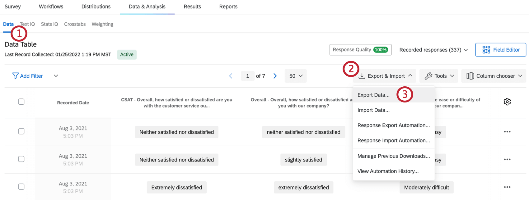
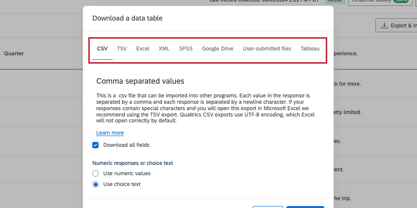
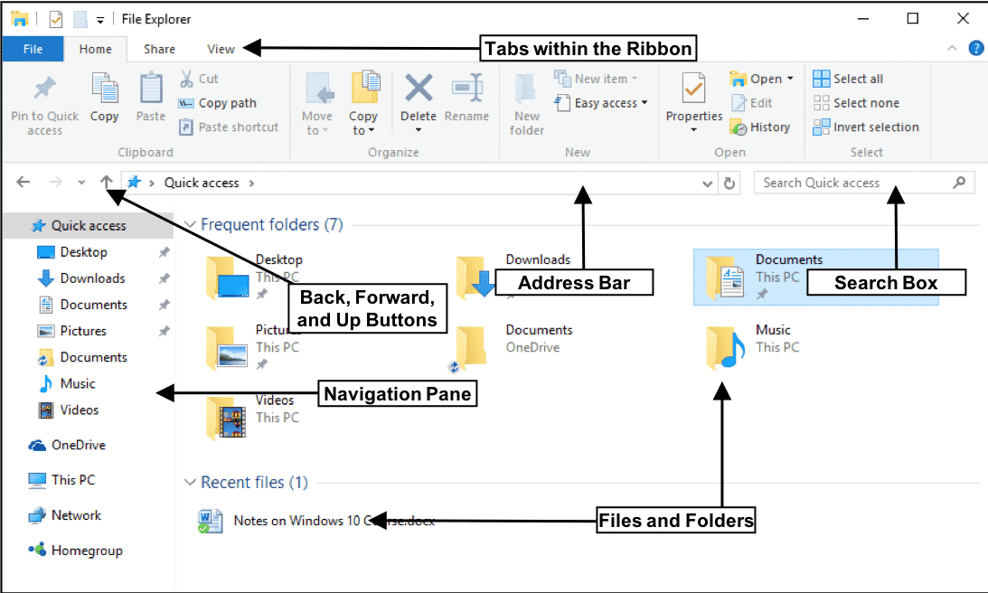
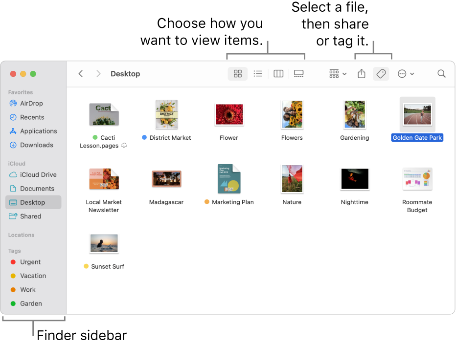
Control where it’s saved!!
Save the data within your papaja project folder:
SPSS
papaja
- Create a “code chunk”:
- Paste the content
## Cynicism

library(dplyr)
library(tidyr)
library(ggplot2)

data <- read.csv("Cynicism Project_April 29, 2025_16.35 2.csv")
names <- data[1,]
names(data) <- names
data <- data[-c(1:2),]

df <- mutate_all(data, function(x) as.numeric(as.character(x)))

reliability <- psych::alpha(df[c(18:31)])  ##

apa_table(reliability$alpha.drop,
          caption="Our reliability analyses",
          note="anything extra here",
          landscape=TRUE,
          font_size='tiny')

hists <- df %>%
        pivot_longer(
          cols="I would describe myself as emotionally stable.":"I prefer my own company to the company of others."
        )

hists2 <- df %>%
        pivot_longer(
          cols="I find it hard to trust those I am close to.":"Others perceive me as moody."
        )

ggplot(hists, aes(x=value))+
  geom_histogram(aes(y=..density..,fill=name),color="grey80")+
  facet_grid(name~.)

ggplot(hists2, aes(x=value))+
  geom_histogram(aes(y=..density..,fill=name),color="grey80")+
  facet_grid(name~.)
## Relationship well-being
library(dplyr)
library(tidyr)
library(ggplot2)
data <- read.csv("Cynicism Project_April 29, 2025_16.35 2.csv")
names <- data[1,]
names(data) <- names
data <- data[-c(1:2),]
df <- mutate_all(data, function(x) as.numeric(as.character(x)))
reliability1 <- psych::alpha(df[c(43:60)]) ##
reliability2 <- psych::alpha(df[c(43:45)]) ##
reliability3 <- psych::alpha(df[c(46:48)]) ##
reliability4 <- psych::alpha(df[c(49:51)]) ##
reliability5 <- psych::alpha(df[c(52:54)]) ##
reliability6 <- psych::alpha(df[c(55:57)]) ##
reliability7 <- psych::alpha(df[c(58:60)]) ##
apa_table(reliability1$alpha.drop,
caption="Our overall reliability analyses",
note="anything extra here",
landscape=TRUE,
font_size='tiny')
apa_table(reliability2$alpha.drop,
caption="Forgiveness subscale",
note="anything extra here",
landscape=TRUE,
font_size='tiny')
apa_table(reliability3$alpha.drop,
caption="Conflict Resolution subscale",
note="anything extra here",
landscape=TRUE,
font_size='tiny')
apa_table(reliability4$alpha.drop,
caption="Trust subscale",
note="anything extra here",
landscape=TRUE,
font_size='tiny')
apa_table(reliability5$alpha.drop,
caption="Respect subscale",
note="anything extra here",
landscape=TRUE,
font_size='tiny')
apa_table(reliability6$alpha.drop,
caption="Kindness subscale",
note="anything extra here",
landscape=TRUE,
font_size='tiny')
apa_table(reliability7$alpha.drop,
caption="Intimacy subscale",
note="anything extra here",
landscape=TRUE,
font_size='tiny')
hists <- df %>%
pivot_longer(
cols="Trust - I can share anything with my partner without fear of judgement.":"Intimacy - I am uncomfortable expressing my true thoughts and emotions to my partner."
)
hists2 <- df %>%
pivot_longer(
cols="Forgiveness - My partner tends to hold grudges against me.":"Trust - I feel emotionally safe in my relationship."
)
ggplot(hists, aes(x=value))+
geom_histogram(aes(y=..density..,fill=name),color="grey80")+
facet_grid(name~.)
ggplot(hists2, aes(x=value))+
geom_histogram(aes(y=..density..,fill=name),color="grey80")+
facet_grid(name~.)## Sense of humor
library(dplyr)
library(tidyr)
library(ggplot2)
data <- read.csv("Commitment to Social Change & Humor_April 24, 2025_17.03.csv")
names <- data[1,]
names(data) <- names
data <- data[-c(1:2),]
df <- mutate_all(data, function(x) as.numeric(as.character(x)))
reliability <- psych::alpha(df[c(34:57)]) ## combined -- different items in different surveys?
apa_table(reliability$alpha.drop,
caption="Our reliability analyses",
note="anything extra here",
landscape=TRUE,
font_size='tiny')
hists <- df %>%
pivot_longer(
cols="I am the funniest person in my friendgroup":"Some people can be \"too funny\""
)
hists2 <- df %>%
pivot_longer(
cols="Jokes at another person's expense are never okay":"I have an a unique sense of humor"
)
hists3 <- df %>%
pivot_longer(
cols="I often find things funny when I’m alone":"I find it annoying when people joke too much"
)
ggplot(hists, aes(x=value))+
geom_histogram(aes(y=..density..,fill=name),color="grey80")+
facet_grid(name~.)
ggplot(hists2, aes(x=value))+
geom_histogram(aes(y=..density..,fill=name),color="grey80")+
facet_grid(name~.)
ggplot(hists3, aes(x=value))+
geom_histogram(aes(y=..density..,fill=name),color="grey80")+
facet_grid(name~.)## Oppression based strain
library(dplyr)
library(tidyr)
library(ggplot2)
data <- read.csv("Humor & Oppression-Based Strain_April 29, 2025_16.40.csv")
names <- data[1,]
names2 <- stringr::str_replace(names, "Rate the following statements to the best of your ability.","")
names(data) <- names2
data <- data[-c(1:2),]
df <- mutate_all(data, function(x) as.numeric(as.character(x)))
reliability1 <- psych::alpha(df[c(66:78)]) ##
apa_table(reliability1$alpha.drop,
caption="Our overall reliability analyses",
note="anything extra here",
landscape=TRUE,
align = c("p{10cm}", rep("p{1cm}",8)),
font_size='tiny')
hists <- df %>%
pivot_longer(
cols=" - Because of my identity I feel excluded from my society":" - Because of my identity I may be discriminated against by hospital staff, my general practitioner, my workplace, or my friends"
)
hists2 <- df %>%
pivot_longer(
cols=" - Because of my identity I have been the target of verbal aggressions.":" - Because of my identity I expect to be the target of insults"
)
ggplot(hists, aes(x=value))+
geom_histogram(aes(y=..density..,fill=name),color="grey80")+
facet_grid(name~.)
ggplot(hists2, aes(x=value))+
geom_histogram(aes(y=..density..,fill=name),color="grey80")+
facet_grid(name~.)## Commitment to Social Change
library(dplyr)
library(tidyr)
library(ggplot2)
data <- read.csv("data.csv")
names <- data[1,]
names(data) <- names
data <- data[-c(1:2),]
df <- mutate_all(data, function(x) as.numeric(as.character(x)))
reliability1 <- psych::alpha(df[c(19:33)]) ##
apa_table(reliability1$alpha.drop,
caption="Our overall reliability analyses",
note="anything extra here",
landscape=TRUE,
align = c("p{10cm}", rep("p{1cm}",8)),
font_size='tiny')
hists <- df %>%
pivot_longer(
cols="I feel marches/boycotts/protests/etc. are effective means of social change.":"I express my opinion about political issues or organizations when I am with friends"
)
hists2 <- df %>%
pivot_longer(
cols="Indicate to what extent you agree or disagree with the following statements:\nIt takes too much effort to engage in activism and advocacy.":"There is someone else who can handle the issues in the world."
)
ggplot(hists, aes(x=value))+
geom_histogram(aes(y=..density..,fill=name),color="grey80")+
facet_grid(name~.)
ggplot(hists2, aes(x=value))+
geom_histogram(aes(y=..density..,fill=name),color="grey80")+
facet_grid(name~.)

SPSS Analyses
** Relationship well-being

GET
  FILE='C:\Users\foss5527\OneDrive - University of St. Thomas\Desktop\data.sav'.

** individual item histograms.

GRAPH
  /HISTOGRAM(NORMAL)=Q36_1.

GRAPH
  /HISTOGRAM(NORMAL)=Q36_2.

GRAPH
  /HISTOGRAM(NORMAL)=Q36_3.

GRAPH
  /HISTOGRAM(NORMAL)=Q41_1.

GRAPH
  /HISTOGRAM(NORMAL)=Q41_2.

GRAPH
  /HISTOGRAM(NORMAL)=Q41_3.

GRAPH
  /HISTOGRAM(NORMAL)=Q38_1.

GRAPH
  /HISTOGRAM(NORMAL)=Q38_2.

GRAPH
  /HISTOGRAM(NORMAL)=Q38_3.

GRAPH
  /HISTOGRAM(NORMAL)=Q37_1.

GRAPH
  /HISTOGRAM(NORMAL)=Q37_2.

GRAPH
  /HISTOGRAM(NORMAL)=Q37_3.

GRAPH
  /HISTOGRAM(NORMAL)=Q39_1.

GRAPH
  /HISTOGRAM(NORMAL)=Q39_2.

GRAPH
  /HISTOGRAM(NORMAL)=Q39_3.

GRAPH
  /HISTOGRAM(NORMAL)=Q40_1.

GRAPH
  /HISTOGRAM(NORMAL)=Q40_2.

GRAPH
  /HISTOGRAM(NORMAL)=Q40_3.


** recodes for reverse-scored items.

RECODE Q41_3 Q39_3 Q40_3 (1=5) (2=4) (4=2) (5=1).
EXECUTE.

** alpha and corrected item-total correlations.

RELIABILITY
  /VARIABLES=Q36_1 Q36_2 Q36_3 Q41_1 Q41_2 Q41_3 Q38_1 Q38_2 Q38_3 Q37_1 Q37_2 Q37_3 Q39_1 Q39_2
    Q39_3 Q40_1 Q40_2 Q40_3
  /SCALE('ALL VARIABLES') ALL
  /MODEL=ALPHA
  /STATISTICS=DESCRIPTIVE SCALE
  /SUMMARY=TOTAL.

** Aggregate scale score across items.

COMPUTE overall=MEAN(Q36_1, Q36_2, Q36_3, Q41_1, Q41_2, Q41_3, Q38_1, Q38_2, Q38_3, Q37_1, Q37_2, Q37_3, Q39_1, Q39_2, Q39_3, Q40_1, Q40_2, Q40_3).
EXECUTE.

** frequency distribution of our measure.

GRAPH
  /HISTOGRAM(NORMAL)=overall.

*** this is our convergent measure, recode and scale score

RECODE Q43_1, Q43_2, Q43_7 (1=5) (2=4) (4=2) (5=1).
EXECUTE.

COMPUTE quality=MEAN(Q43_1, Q43_2, Q43_3, Q43_4, Q43_5, Q43_6, Q43_7, Q43_8, Q43_9, Q43_10, Q43_11).
EXECUTE.

** frequency distribution of convergent measure.

GRAPH
  /HISTOGRAM(NORMAL)=quality.

** Convergent validity index.

CORRELATIONS
  /VARIABLES=overall quality
  /PRINT=TWOTAIL NOSIG FULL
  /MISSING=PAIRWISE.
** Sense of humor.
GET
FILE='C:\Users\juar6666\OneDrive - University of St. Thomas\Desktop\DATA.sav'.
** reflecting item responses.
RECODE Q55 Q59 Q5.0 Q6 Q53 Q7 Q10 Q49 Q52 Q54 (1=4) (2=3) (3=2) (4=1).
EXECUTE.
** trying to rescue items that "work".
CORRELATIONS
/VARIABLES=Q9 Q50 Q6 QID1 Q2 Q55 Q59 Q3 Q4 Q5.0 Q57
/PRINT=TWOTAIL NOSIG FULL
/MISSING=PAIRWISE.
** testing reliability of subset of items.
RELIABILITY
/VARIABLES= Q6 Q9 Q50
/SCALE('ALL VARIABLES') ALL
/MODEL=ALPHA
/STATISTICS=DESCRIPTIVE SCALE
/SUMMARY=TOTAL.
** individual item histograms.
GRAPH
/HISTOGRAM(NORMAL)=QID1.
GRAPH
/HISTOGRAM(NORMAL)=Q2.
GRAPH
/HISTOGRAM(NORMAL)=Q55.
GRAPH
/HISTOGRAM(NORMAL)=Q59.
GRAPH
/HISTOGRAM(NORMAL)=Q3.
GRAPH
/HISTOGRAM(NORMAL)=Q4.
GRAPH
/HISTOGRAM(NORMAL)=Q5.0.
GRAPH
/HISTOGRAM(NORMAL)=Q57.
GRAPH
/HISTOGRAM(NORMAL)=Q6.
GRAPH
/HISTOGRAM(NORMAL)=Q53.
GRAPH
/HISTOGRAM(NORMAL)=Q7.
GRAPH
/HISTOGRAM(NORMAL)=Q58.
GRAPH
/HISTOGRAM(NORMAL)=Q8.
GRAPH
/HISTOGRAM(NORMAL)=Q9.
GRAPH
/HISTOGRAM(NORMAL)=Q10.
GRAPH
/HISTOGRAM(NORMAL)=Q46.
GRAPH
/HISTOGRAM(NORMAL)=Q56.
GRAPH
/HISTOGRAM(NORMAL)=Q47.
GRAPH
/HISTOGRAM(NORMAL)=Q48.
GRAPH
/HISTOGRAM(NORMAL)=Q49.
GRAPH
/HISTOGRAM(NORMAL)=Q50.
GRAPH
/HISTOGRAM(NORMAL)=Q51.
GRAPH
/HISTOGRAM(NORMAL)=Q52.
GRAPH
/HISTOGRAM(NORMAL)=Q54.
GRAPH
/HISTOGRAM(NORMAL)=Q12.
GRAPH
/HISTOGRAM(NORMAL)=Q13.
GRAPH
/HISTOGRAM(NORMAL)=Q14.
GRAPH
/HISTOGRAM(NORMAL)=Q16.
GRAPH
/HISTOGRAM(NORMAL)=Q17.
GRAPH
/HISTOGRAM(NORMAL)=Q18.
GRAPH
/HISTOGRAM(NORMAL)=Q19.
GRAPH
/HISTOGRAM(NORMAL)=Q20.
GRAPH
/HISTOGRAM(NORMAL)=Q21.
GRAPH
/HISTOGRAM(NORMAL)=Q23.
GRAPH
/HISTOGRAM(NORMAL)=Q24.
GRAPH
/HISTOGRAM(NORMAL)=Q25.
GRAPH
/HISTOGRAM(NORMAL)=Q26.
GRAPH
/HISTOGRAM(NORMAL)=Q27.
GRAPH
/HISTOGRAM(NORMAL)=Q28.
GRAPH
/HISTOGRAM(NORMAL)=Q29.
GRAPH
/HISTOGRAM(NORMAL)=Q30.
GRAPH
/HISTOGRAM(NORMAL)=Q31.
GRAPH
/HISTOGRAM(NORMAL)=Q32.
GRAPH
/HISTOGRAM(NORMAL)=Q33.0.
GRAPH
/HISTOGRAM(NORMAL)=Q34.
GRAPH
/HISTOGRAM(NORMAL)=Q35.
** SCALE score - should be consistent with reliability analysis items.
COMPUTE Humor=MEAN(QID1,Q2,Q55,Q59,Q3,Q4,Q5.0,Q57,Q6,Q53,Q7,Q58,Q8,Q9,Q10,Q46,Q56,Q47,Q48,Q49,Q50,Q51,Q52,Q54).
EXECUTE.
COMPUTE Humor2=MEAN(Q12,Q13,Q14,Q16,Q17,Q18,Q19,Q20,Q21,Q23,Q24,Q25,Q26,Q27,Q28,Q29,Q30,Q31,Q32,Q33,Q34,Q35).
EXECUTE.
** frequency distributions of scale scores (ours and convergent).
GRAPH
/HISTOGRAM(NORMAL)=Humor2.
GRAPH
/HISTOGRAM(NORMAL)=Humor.
** convergent validity coefficient.
CORRELATIONS
/VARIABLES=Humor2 Humor
/PRINT=TWOTAIL NOSIG FULL
/MISSING=PAIRWISE.** Oppression based strain.
GET
FILE='C:\Users\juar6666\OneDrive - University of St. Thomas\Desktop\DATA.sav'.
**reverse both for our and covnergent measure 19-31
RECODE Q55 Q59 Q5.0 Q6 Q53 Q7 Q10 Q49 Q52 Q19 Q24 Q28 Q31 (1=4) (2=3) (3=2) (4=1).
EXECUTE.
** looking at assignment 3 analyses.
** individual item histograms first.
GRAPH
/HISTOGRAM(NORMAL)=Q1_1.
GRAPH
/HISTOGRAM(NORMAL)=Q1_2.
GRAPH
/HISTOGRAM(NORMAL)=Q1_3.
GRAPH
/HISTOGRAM(NORMAL)=Q1_1.0.
GRAPH
/HISTOGRAM(NORMAL)=Q1_2.0.
GRAPH
/HISTOGRAM(NORMAL)=Q1_3.0.
GRAPH
/HISTOGRAM(NORMAL)=Q1_1.1.
GRAPH
/HISTOGRAM(NORMAL)=Q1_2.1.
GRAPH
/HISTOGRAM(NORMAL)=Q1_3.1.
GRAPH
/HISTOGRAM(NORMAL)=Q1_1.2.
GRAPH
/HISTOGRAM(NORMAL)=Q1_2.2.
GRAPH
/HISTOGRAM(NORMAL)=Q1_3.2.
GRAPH
/HISTOGRAM(NORMAL)=Q1_1.3.
GRAPH
/HISTOGRAM(NORMAL)=Q1_2.3.
GRAPH
/HISTOGRAM(NORMAL)=Q1_3.3.
GRAPH
/HISTOGRAM(NORMAL)=Q1_1.4.
GRAPH
/HISTOGRAM(NORMAL)=Q1_2.4.
GRAPH
/HISTOGRAM(NORMAL)=Q1_3.4.
** Strain alpha (subscale).
RELIABILITY
/VARIABLES=Q1_1 Q1_2 Q1_3 Q1_1.0 Q1_2.0 Q1_3.0 Q1_1.1 Q1_2.1 Q1_3.1 Q1_1.2 Q1_2.2 Q1_3.2
/SCALE('Strain Alpha') ALL
/MODEL=ALPHA
/STATISTICS=DESCRIPTIVE SCALE
/SUMMARY=TOTAL.
** Oppression alpha (subscale).
RELIABILITY
/VARIABLES=Q1_1.3 Q1_2.3 Q1_3.3 Q1_1.4 Q1_2.4 Q1_3.4
/SCALE('Oppression Alpha') ALL
/MODEL=ALPHA
/STATISTICS=DESCRIPTIVE SCALE
/SUMMARY=TOTAL.
** Oppression-based strain alpha (Overall/Combined).
RELIABILITY
/VARIABLES=Q1_1 Q1_2 Q1_3 Q1_1.0 Q1_2.0 Q1_3.0 Q1_1.1 Q1_2.1 Q1_3.1 Q1_1.2 Q1_2.2 Q1_3.2 Q1_1.3
Q1_2.3 Q1_3.3 Q1_1.4 Q1_2.4 Q1_3.4
/SCALE('Oppression-Based Strain Alpha') ALL
/MODEL=ALPHA
/STATISTICS=DESCRIPTIVE SCALE
/SUMMARY=TOTAL.
** Strain (sub)scale score.
COMPUTE Strain=MEAN(Q1_1,Q1_2,Q1_3,Q1_1.0,Q1_2.0,Q1_3.0,Q1_1.1,Q1_2.1,Q1_3.1,Q1_1.2,Q1_2.2,Q1_3.2).
EXECUTE.
*Oppression (sub)scale score.
COMPUTE Oppression=MEAN(Q1_1.3,Q1_2.3,Q1_3.3,Q1_1.4,Q1_2.4,Q1_3.4).
EXECUTE.
*Oppresion based strain scale score.
COMPUTE OppressionBasedStrain=MEAN(Q1_3.4,Q1_2.4,Q1_1.4,Q1_3.3,Q1_2.3,Q1_1.3,Q1_3.2,Q1_3.2,Q1_2.2,
Q1_1.2,Q1_3.1,Q1_2.1,Q1_1.1,Q1_3.0,Q1_2.0,Q1_1.0,Q1_3,Q1_2,Q1_1).
EXECUTE.
** Scale frequency distributions.
GRAPH
/HISTOGRAM(NORMAL)=Strain.
GRAPH
/HISTOGRAM(NORMAL)=Oppression.
GRAPH
/HISTOGRAM(NORMAL)=OppressionBasedStrain.
** correlation between subscales.
GRAPH
/SCATTERPLOT(BIVAR)=Oppression WITH Strain
/MISSING=LISTWISE.** Commitment to Social Change
** grabbing .csv data - make sure to double check "AUTO" variable name changes
GET DATA /TYPE=TXT
/FILE="C:\Users\ries6020\OneDrive - University of St. Thomas\data.csv"
/ENCODING='UTF8'
/DELCASE=LINE
/DELIMITERS=" ;,"
/QUALIFIER='"'
/ARRANGEMENT=DELIMITED
/FIRSTCASE=16
/DATATYPEMIN PERCENTAGE=95.0
/VARIABLES=
StartDate AUTO
EndDate AUTO
Status AUTO
IPAddress AUTO
Progress AUTO
Duration AUTO
in AUTO
seconds AUTO
Finished AUTO
RecordedDate AUTO
ResponseId AUTO
RecipientLastName AUTO
RecipientFirstName AUTO
RecipientEmail AUTO
ExternalReference AUTO
LocationLatitude AUTO
LocationLongitude AUTO
DistributionChannel AUTO
UserLanguage AUTO
QID7 AUTO
Q1_1 AUTO
Q2_1 AUTO
Q3_1 AUTO
Q4_1 AUTO
Q5_1 AUTO
Q6_1 AUTO
Q7_1 AUTO
Q8_1 AUTO
Q9_1 AUTO
Q10_1 AUTO
Q11_1 AUTO
Q12_1 AUTO
Q13_1 AUTO
Q14_1 AUTO
Q15_1 AUTO
Q16 AUTO
Q17 AUTO
Q18 AUTO
Q19 AUTO
Q20 AUTO
Q21 AUTO
Q22 AUTO
Q23 AUTO
Q24 AUTO
Q25 AUTO
Q26 AUTO
Q27 AUTO
Q28 AUTO
Q29 AUTO
Q30 AUTO
Q31 AUTO
Q32 AUTO
Q33 AUTO
Q34 AUTO
Q35 AUTO
Q36 AUTO
Q37 AUTO
Q38 AUTO
Q39 AUTO
Q40 AUTO
Q41 AUTO
Q41_10_TEXT AUTO
Q42 AUTO
Q42_7_TEXT AUTO
Q43 AUTO
Q44 AUTO
V67 AUTO
V68 AUTO
V69 AUTO
V70 AUTO
V71 AUTO
V72 AUTO
V73 AUTO
V74 AUTO
V75 AUTO
V76 AUTO
V77 AUTO
V78 AUTO
V79 AUTO
V80 AUTO
V81 AUTO
V82 AUTO
V83 AUTO
V84 AUTO
V85 AUTO
V86 AUTO
V87 AUTO
V88 AUTO
V89 AUTO
V90 AUTO
V91 AUTO
V92 AUTO
V93 AUTO
V94 AUTO
V95 AUTO
V96 AUTO
V97 AUTO
V98 AUTO
V99 AUTO
V100 AUTO
V101 AUTO
V102 AUTO
V103 AUTO
/MAP.
EXECUTE.
** Convergent measure (5 items, none reflected)
COMPUTE convergent_social=MEAN(Q11_1, Q12_1, Q13_1, Q14_1, Q15_1).
EXECUTE.
*** reflecting responses to 4 reverse keyed items (our scale)
RECODE Q6_1 Q1_1 Q4_1 Q8_1 (1=5) (2=4) (4=2) (5=1).
EXECUTE.
COMPUTE our_social=MEAN(Q1_1, Q2_1, Q3_1, Q4_1, Q5_1, Q5_1, Q6_1, Q7_1, Q8_1, Q9_1, Q10_1).
EXECUTE.
CORRELATIONS
/VARIABLES=convergent_social our_social
/PRINT=ONETAIL NOSIG FULL
/MISSING=PAIRWISE.Peer Evaluations
Dimensions:
- Responsibility – fully assuming role as team member & committing to all tasks that are a part of the project (k=5)
- Communication – ability to communicate in a productive and timely manner (k=5)
- Dependability – actions consistently matching words (k=5)
- Flexibility – ability to adapt to changes throughout the project (k=5)
- Teamwork – ability to compromise and/or successfully navigate disagreements when working as a group (k=5)
preview available here

