Dealing with Data
TODAY!! (5/13)
- group project teams
- compute scale scores
- YOUR measure
- your convergent measure
- reverse–score if needed
- share SPSS syntax with discriminant group
Note
For presentation, only a brief summary is necessary1, but be prepared for questions (that you will put into paper)

Sona Timeslots
- Log in to Sona
- Choose your study (
My Studies) - Click on
Add A Timeslot Number of Participants= 200Researcherdoesn’t matter – it’s online


Accessing data from Qualtrics
- find “Data” tab in
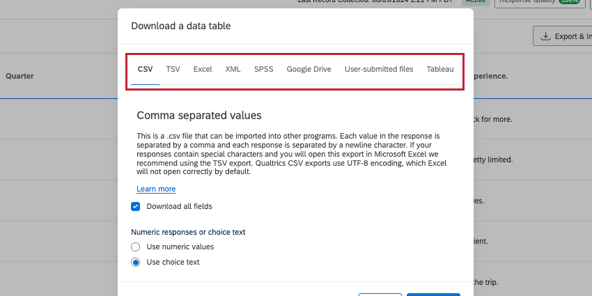
Data & Analysissection - export responses as “CSV”
- select “numeric values”
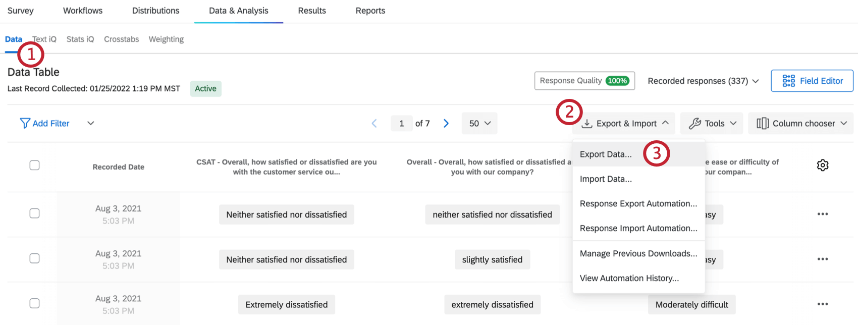
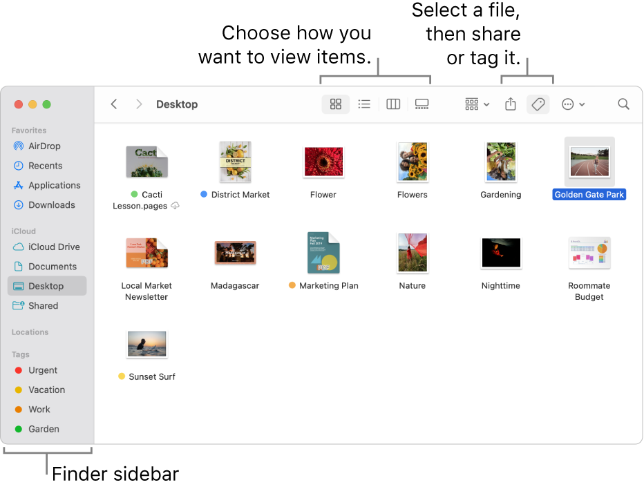
Control where it’s saved!!
Save the data within your papaja project folder:

SPSS
- Open SPSS
File\(\rightarrow\)Import Data1Pasteinto a syntax file- Save the syntax file within your
papajafolder

papaja
- Create a “code chunk”:

- Paste the content
## Cynicism

library(dplyr)
library(tidyr)
library(ggplot2)

data <- read.csv("Cynicism Project_April 29, 2025_16.35 2.csv")
names <- data[1,]
names(data) <- names
data <- data[-c(1:2),]

df <- mutate_all(data, function(x) as.numeric(as.character(x)))

reliability <- psych::alpha(df[c(18:31)])  ##

apa_table(reliability$alpha.drop,
          caption="Our reliability analyses",
          note="anything extra here",
          landscape=TRUE,
          font_size='tiny')

hists <- df %>%
        pivot_longer(
          cols="I would describe myself as emotionally stable.":"I prefer my own company to the company of others."
        )

hists2 <- df %>%
        pivot_longer(
          cols="I find it hard to trust those I am close to.":"Others perceive me as moody."
        )

ggplot(hists, aes(x=value))+
  geom_histogram(aes(y=..density..,fill=name),color="grey80")+
  facet_grid(name~.)

ggplot(hists2, aes(x=value))+
  geom_histogram(aes(y=..density..,fill=name),color="grey80")+
  facet_grid(name~.)
## Relationship well-being
library(dplyr)
library(tidyr)
library(ggplot2)
data <- read.csv("Cynicism Project_April 29, 2025_16.35 2.csv")
names <- data[1,]
names(data) <- names
data <- data[-c(1:2),]
df <- mutate_all(data, function(x) as.numeric(as.character(x)))
reliability1 <- psych::alpha(df[c(43:60)]) ##
reliability2 <- psych::alpha(df[c(43:45)]) ##
reliability3 <- psych::alpha(df[c(46:48)]) ##
reliability4 <- psych::alpha(df[c(49:51)]) ##
reliability5 <- psych::alpha(df[c(52:54)]) ##
reliability6 <- psych::alpha(df[c(55:57)]) ##
reliability7 <- psych::alpha(df[c(58:60)]) ##
apa_table(reliability1$alpha.drop,
caption="Our overall reliability analyses",
note="anything extra here",
landscape=TRUE,
font_size='tiny')
apa_table(reliability2$alpha.drop,
caption="Forgiveness subscale",
note="anything extra here",
landscape=TRUE,
font_size='tiny')
apa_table(reliability3$alpha.drop,
caption="Conflict Resolution subscale",
note="anything extra here",
landscape=TRUE,
font_size='tiny')
apa_table(reliability4$alpha.drop,
caption="Trust subscale",
note="anything extra here",
landscape=TRUE,
font_size='tiny')
apa_table(reliability5$alpha.drop,
caption="Respect subscale",
note="anything extra here",
landscape=TRUE,
font_size='tiny')
apa_table(reliability6$alpha.drop,
caption="Kindness subscale",
note="anything extra here",
landscape=TRUE,
font_size='tiny')
apa_table(reliability7$alpha.drop,
caption="Intimacy subscale",
note="anything extra here",
landscape=TRUE,
font_size='tiny')
hists <- df %>%
pivot_longer(
cols="Trust - I can share anything with my partner without fear of judgement.":"Intimacy - I am uncomfortable expressing my true thoughts and emotions to my partner."
)
hists2 <- df %>%
pivot_longer(
cols="Forgiveness - My partner tends to hold grudges against me.":"Trust - I feel emotionally safe in my relationship."
)
ggplot(hists, aes(x=value))+
geom_histogram(aes(y=..density..,fill=name),color="grey80")+
facet_grid(name~.)
ggplot(hists2, aes(x=value))+
geom_histogram(aes(y=..density..,fill=name),color="grey80")+
facet_grid(name~.)## Sense of humor
library(dplyr)
library(tidyr)
library(ggplot2)
data <- read.csv("Commitment to Social Change & Humor_April 24, 2025_17.03.csv")
names <- data[1,]
names(data) <- names
data <- data[-c(1:2),]
df <- mutate_all(data, function(x) as.numeric(as.character(x)))
reliability <- psych::alpha(df[c(34:57)]) ## combined -- different items in different surveys?
apa_table(reliability$alpha.drop,
caption="Our reliability analyses",
note="anything extra here",
landscape=TRUE,
font_size='tiny')
hists <- df %>%
pivot_longer(
cols="I am the funniest person in my friendgroup":"Some people can be \"too funny\""
)
hists2 <- df %>%
pivot_longer(
cols="Jokes at another person's expense are never okay":"I have an a unique sense of humor"
)
hists3 <- df %>%
pivot_longer(
cols="I often find things funny when I’m alone":"I find it annoying when people joke too much"
)
ggplot(hists, aes(x=value))+
geom_histogram(aes(y=..density..,fill=name),color="grey80")+
facet_grid(name~.)
ggplot(hists2, aes(x=value))+
geom_histogram(aes(y=..density..,fill=name),color="grey80")+
facet_grid(name~.)
ggplot(hists3, aes(x=value))+
geom_histogram(aes(y=..density..,fill=name),color="grey80")+
facet_grid(name~.)## Oppression based strain
library(dplyr)
library(tidyr)
library(ggplot2)
data <- read.csv("Humor & Oppression-Based Strain_April 29, 2025_16.40.csv")
names <- data[1,]
names2 <- stringr::str_replace(names, "Rate the following statements to the best of your ability.","")
names(data) <- names2
data <- data[-c(1:2),]
df <- mutate_all(data, function(x) as.numeric(as.character(x)))
reliability1 <- psych::alpha(df[c(66:78)]) ##
apa_table(reliability1$alpha.drop,
caption="Our overall reliability analyses",
note="anything extra here",
landscape=TRUE,
align = c("p{10cm}", rep("p{1cm}",8)),
font_size='tiny')
hists <- df %>%
pivot_longer(
cols=" - Because of my identity I feel excluded from my society":" - Because of my identity I may be discriminated against by hospital staff, my general practitioner, my workplace, or my friends"
)
hists2 <- df %>%
pivot_longer(
cols=" - Because of my identity I have been the target of verbal aggressions.":" - Because of my identity I expect to be the target of insults"
)
ggplot(hists, aes(x=value))+
geom_histogram(aes(y=..density..,fill=name),color="grey80")+
facet_grid(name~.)
ggplot(hists2, aes(x=value))+
geom_histogram(aes(y=..density..,fill=name),color="grey80")+
facet_grid(name~.)## Commitment to Social Change
library(dplyr)
library(tidyr)
library(ggplot2)
data <- read.csv("data.csv")
names <- data[1,]
names(data) <- names
data <- data[-c(1:2),]
df <- mutate_all(data, function(x) as.numeric(as.character(x)))
reliability1 <- psych::alpha(df[c(19:33)]) ##
apa_table(reliability1$alpha.drop,
caption="Our overall reliability analyses",
note="anything extra here",
landscape=TRUE,
align = c("p{10cm}", rep("p{1cm}",8)),
font_size='tiny')
hists <- df %>%
pivot_longer(
cols="I feel marches/boycotts/protests/etc. are effective means of social change.":"I express my opinion about political issues or organizations when I am with friends"
)
hists2 <- df %>%
pivot_longer(
cols="Indicate to what extent you agree or disagree with the following statements:\nIt takes too much effort to engage in activism and advocacy.":"There is someone else who can handle the issues in the world."
)
ggplot(hists, aes(x=value))+
geom_histogram(aes(y=..density..,fill=name),color="grey80")+
facet_grid(name~.)
ggplot(hists2, aes(x=value))+
geom_histogram(aes(y=..density..,fill=name),color="grey80")+
facet_grid(name~.)
![]()