This tutorial reviews some concepts using the econometrics software package R. Specifically, the tutorial reviews:
Pooled OLS model. with cluster-robust standard errors
Fixed Effects (Within Estimator), with cluster-robust standard errors
Random Effects, with cluster robust standard errors
Correlated Random Effects (CRE), with cluster robust standard errors
This tutorial requires one (1) data file:
tut12_panel.csv
This file can be obtained from the Canvas subject page
In addition, the file, tut12.R , provides the program code (R script file) necessary to complete this tutorial. The R script file uses the following packages which need to be installed prior to running this program:
stargazer :
for easily generating summary statistics for an R data file
ggplot2 :
for easily producing graphs in R
car:
for easily conducting hypothesis tests in R
lmtest :
for easily conducting the Ramsey RESET test in R
sandwich:
for easily calculating robust standard errors in R
rio:
for easily importing data into R
plm:
for easily estimating models linear panel data models in R
These can be installed directly in RStudio from the packages tab or by using the command install.packages() and inserting the name of the package in the brackets.
Question
Consider the following econometric model for the price of airline seats on routes in a large country: \[\begin{align}
\ln\,\mbox{fare}_{it} & = \beta_{0} + \beta_{1}\,\mbox{concen}_{it} + \beta_{2}\,\ln\,\mbox{dist}_{i} + \beta_{3}\left\{\ln\,\mbox{dist}_{i}\right\}^{2} \notag \\
& + \beta_{4}\,\mbox{YEAR1998}_{t} + \beta_{5}\,\mbox{YEAR1999}_{t} + \beta_{6}\,\mbox{YEAR2000}_{t} + \varepsilon_{it}
\tag{1}
\end{align}\] with the following assumptions
where: \[\begin{align*}
\text{fare}_{it} = & \mbox{ average fare on route $i$ in period $t$, in dollars} \\
\text{dist}_{i} = & \mbox{ average distance of route $i$, in miles} \\
\text{concen}_{it} = & \mbox{ market concentration, measured by the market share of the largest carrier} \\
& \mbox{ on route $i$ at time $t$} \\
\text{YEAR1998}_{t} = & \mbox{ 1 if year=1998, 0 otherwise} \\
\text{YEAR1999}_{t} = & \mbox{ 1 if year=1999, 0 otherwise} \\
\text{YEAR2000}_{t} = & \mbox{ 1 if year=2000, 0 otherwise} \\
\end{align*}\] and \(\ln(X)\) denotes the natural logarithm of variable \(X\).
The data file tut12_panel.csv contains observations on 1,149 airline routes for the period 1997 - 2000.
(a)
Estimate the econometric model (1) by Ordinary Least Squares (OLS).
The estimation results are reported in Figure 1. As the assumptions are written, the OLS estimator for model (1) will be a consistent estimator of the population parameters. However, the sample consists of repeated observations on airline routes. The assumptions about the error terms outlined above may not necessarily be appropriate. It is likely that the errors are correlated over time, for each route. In this case, the error \(\varepsilon_{it}\) might be characterised by both heteroskedasticity and autocorrelation, within routes.
In this case, the OLS estimator will still be consistent but the standard errors will be wrong. Conclusions based upon t-tests and F-tests could provide misleading conclusions.
(b)
Do you think that the standard errors are valid? Clearly explain why or why not?
Solution
The estimation results are reported in Figure 1. The following table summarizes the results.
Pooled OLS Ordinary s.e
Pooled OLS Cluster s.e
Variable
coef.
std. error
coef.
std,error
CONCEN
0.3601
0.0301
0.3601
0.0586
LDIST
-1.002
0.1375
-1.002
0.2912
LDISTSQ
0.1031
0.0097
0.1031
0.202
Y98
0.0211
0.0140
0.0211
0.0041
Y99
0.0378
0.0140
0.0378
0.0052
Y00
0.0999
0.0140
0.0999
0.0056
As expected, the (ordinary) OLS standard errors are too low in the presence of errors that are correlated over time, for each route. Note that, for reasons outside the scope of this subject, care must be exercised when using the cluster-robust standard errors on indicator variables (such as the time indicator variables used here). In this example, the cluster-robust standard errors are lower than the (ordinary) OLS standard errors for the time indicator variables.
(c)
Consider the following alternative econometric model: \[\begin{align}
\ln\,\mbox{fare}_{it} & = \beta_{1}\,\mbox{concen}_{it} + \beta_{2}\,\ln\,\mbox{dist}_{i} + \beta_{3}\left\{\ln\,\mbox{dist}_{i}\right\}^{2} \notag \\
& + \beta_{4}\,\mbox{YEAR1998}_{t} + \beta_{5}\,\mbox{YEAR1999}_{t} + \beta_{6}\,\mbox{YEAR2000}_{t} + \upsilon_{i} + \varepsilon_{it}
\tag{2}
\end{align}\] where \(\upsilon_{i}\) represents an unobserved time-invariant random variable and:
\[\begin{align*}
E[\varepsilon_{it}|\mathbf{X}_{it},\upsilon_{i}] =0 & \quad \text{(zero conditional mean)} \\
\mathop{\mathrm{VAR}}[\varepsilon_{it}|\mathbf{X}_{it},\upsilon_{i}] = \sigma^{2} & \quad \text{(homoskedasticity)} \\
\mathop{\mathrm{COV}}[\varepsilon_{it},\,\varepsilon_{is}|\mathbf{X},\upsilon_{i}] = 0 \text{ for } t \ne s & \quad \text{(uncorrelated errors, within groups)} \\
\mathop{\mathrm{COV}}[\varepsilon_{it},\,\varepsilon_{js}|\mathbf{X},\upsilon_{i}] = 0 \text{ for }i \ne j & \quad \text{(uncorrelated errors, across groups)} \\
\mathop{\mathrm{COV}}[\varepsilon_{it},\,\mathbf{X}_{it}|\upsilon_{i}] = 0 & \quad \text{(strict exogeneity)} \\
\end{align*}\]
(i)
Clearly explain, and provide some examples, whether you think that \(\upsilon_{i}\) is correlated with \(\mbox{concen}_{it}\) or not.
Solution
\(\mathbf{\text{COV}[\upsilon_{i},X_{it}] \neq 0}\) for the pooled OLS model
population
demographics
road and rail alternatives
Factors about the cities near the two airports served by the routes could affect demand for air travel. These factors might include population, average education, the characteristics of employers (size, industry etc. \(\ldots\)), and the quality and feasibility of alternatives such as freeways and rail, just to name a few. Although these factors might be time-varying, over a short period (such as the four years in this sample) these might be approximately constant. Importantly, all these time-invariant factors might reasonably be correlated with \(\mbox{concen}_{it}\), the degree of competition on the route, leading to \(\mathop{\mathrm{COV}}(\mbox{concen}_{it},\upsilon_{i}) \ne 0\).
(ii)
Suppose you attempt to estimate this econometric model using the Fixed Effects (FE) estimator. Clearly explain why your estimated model cannot include the distance variables.
Solution
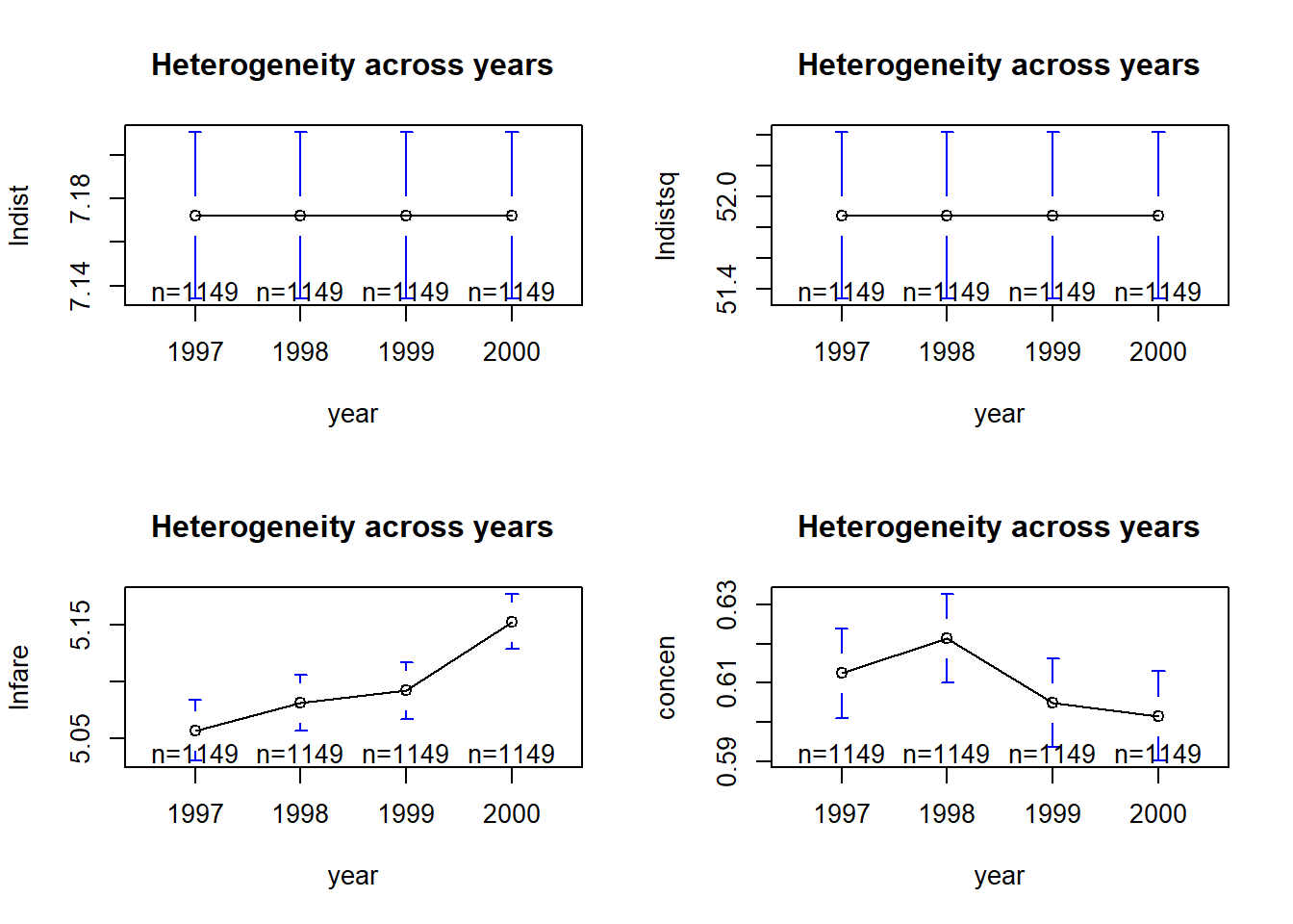
The variables \(\text{lndist}\) and \(\text{lndistsq}\) only vary across routes and not over time, within routes. The “within transformation” applies the following transformation to all variables (to eliminate the fixed effect) - subtract individual specific means from each variable. For example: \(\mbox{lndist}^{*} = \mbox{lndist}{i} - \frac{\sum_{t}\,\mbox{lndist}_{i}}{T} = \mbox{lndist}{i} - \frac{T\,\mbox{lndist}_{i}}{T} = 0\) .The variable \(\text{lndistsq}\) is also transformed in a similar way. Consequently, in a fixed effects specification, the coefficients on time invariant explanatory variables cannot be identified. The fixed effects (FE) estimator only identifies the coefficients using the within-route variation over time.
Fixed Effects Model distance variables are time invariant so are omitted
concentration and log(fare) do vary over time so are included
Code
par(mfrow=c(2,2))library(gplots)plotmeans(lndist~year, main="Heterogeneity across years",data=tut12_pd)plotmeans(lndistsq~year, main="Heterogeneity across years",data=tut12_pd)plotmeans(lnfare~year, main="Heterogeneity across years",data=tut12_pd)plotmeans(concen~year, main="Heterogeneity across years",data=tut12_pd)
(iii)
Estimate model (2) using the Fixed Effects (FE) estimator with cluster-robust standard errors. Compare and contrast the estimate for \(\beta_{1}\) to that obtained for the pooled OLS model in part b).
Solution
Code
#-------------------------------------------# Question (c)(i)-(iv) # Estimate Fixed Effects (FE) model#--------------------------------------# fixed <- plm(lnfare ~ concen + lndist + lndistsq +year1998 + year1999 + year2000, # model="within", data = tut12_pd )# print(summary(fixed))fixed <-plm(lnfare ~ concen + year1998 + year1999 + year2000, model="within", data = tut12_pd )# print(summary(fixed))wald_fixed <-pwaldtest(fixed, test="F")# print(wald_fixed)fstat3 <-round(wald_fixed[[2]][1], digits=4)pvalf3 <-round(wald_fixed[[4]][1], digits=4)numdf3 <-wald_fixed[[3]][1]demdf3 <-wald_fixed[[3]][2]#------------------------------------------# Cluster-Robust Variance Estimator# (1) Use finite Sample: Degrees of Freedom Adjustment# (N/N-1)*(NT-1)*(NT-K-1)# display with cluster VCE and df-adjustmentfixed_crse_vcov <- dfa *vcovHC(fixed, type ="HC0", cluster ="group")fixed_crse_r <-coeftest(fixed, vcov = fixed_crse_vcov)# print(fixed_crse_r)# cluster-robust standard errors for fixed effects modelfixed_crse <-sqrt(diag(fixed_crse_vcov))#---------------------------------------------# Note: pwaldtest reports chi-squared, not F by defaultwald_fixed_crse <-pwaldtest(fixed, vcov = fixed_crse_vcov, test="F")# print(wald_fixed_crse)fstat4 <-round(wald_fixed_crse[[2]][1], digits=4)pvalf4 <-round(wald_fixed_crse[[4]][1], digits=4)numdf4 <-wald_fixed_crse[[3]][1]demdf4 <-wald_fixed_crse[[3]][2]
Code
# compare FE estimator with cluster-robust std. errorsstargazer(fixed,fixed, type ="html", dep.var.labels=c("(Log) Fare"),column.labels =c( "Within", "Within (Cluster-Robust)"),covariate.labels =c("Market Concentration", "Year=1998", "Year=1999", "Year=2000"),se =list(NULL, fixed_crse),omit.stat =c("f","adj.rsq"),add.lines =list(c("F Statistic", fstat3, fstat4),c("F p value", pvalf3, pvalf4),c("F num df", numdf3, numdf4),c("F dem df", demdf3,demdf4)),digits=4, align=TRUE,intercept.bottom=FALSE,star.cutoffs =c(0.05, 0.01, 0.001))
Dependent variable:
(Log) Fare
Within
Within (Cluster-Robust)
(1)
(2)
Market Concentration
0.1689***
0.1689***
(0.0294)
(0.0495)
Year=1998
0.0228***
0.0228***
(0.0045)
(0.0042)
Year=1999
0.0364***
0.0364***
(0.0044)
(0.0051)
Year=2000
0.0978***
0.0978***
(0.0045)
(0.0055)
F Statistic
134.6105
120.004
F p value
0
0
F num df
4
4
F dem df
3443
1148
Observations
4,596
4,596
R2
0.1352
0.1352
Note:
p<0.05; p<0.01; p<0.001
Figure 2: Fixed Effects (Within transformation) Results Model (2)
The estimation results are reported in Figure 2. The OLS results (with cluster-robust standard errors) are compared to the fixed effects estimates in the table below.
Pooled OLS / FE comparison
Relative to FE Pooled OLS suffers from Omitted Variable Bias In FE \(\upsilon_t\) in the error term drops out using the “within transformation”
Pooled OLS Ordinary s.e
Fixed Effects Cluster s.e
Variable
coef.
std. error
coef.
std,error
CONCEN
0.3601
0.0586
0.1689
0.0495
Note the model degrees of freedom for the FE model (without cluster-robust standard errors). The degrees of freedom are \(\left\{NT - (K+1) - (N-1)\right\} = (NT - K - N) (4,596 -4 - 1,149) = 3,443\). The degrees of freedom for the FE model with cluster-robust standard errors is given by \(N-1=1,148\).
Relative to the FE model, the time-invariant unobserved effect \(\upsilon_{i}\) represents an omitted variable in the pooled OLS model. The pooled OLS estimate of 0.3601 is greater than the FE estimate (which controls for \(\upsilon_{i}\)) of 0.1689.
Provided cities with higher values of \(\upsilon_{i}\) tend to have greater fares, this result would be consistent with an omitted variable bias in the pooled OLS model where \(\upsilon_{i}\) is positively correlated with \(\text{concen}_{i}\) - cities with higher values of \(\upsilon_{i}\) tend to also have less competition on air routes (larger market share of largest carriers).
(iv)
At the 5% level of significance, test the hypothesis that the pooled OLS model is the appropriate model, against the alternative that the Fixed Effects Model is the most appropriate. Your answer should clearly state the null and alternative hypothesis, the distribution of the test statistic, and your conclusion.
Test FE vs Pooled OLS
Restricted Model: Pooled OLS Unrestricted: FE (Within) Model not reject \(H_0: \rightarrow\) Pooled OLS reject \(H_0: \rightarrow\) FE model
Solution
The null hypothesis is: \[ H\_{0} : \mbox{’fixed effects’ are jointly } = 0 \qquad H\_{A} : \mbox{at least one ’fixed effect’ } \ne 0 \] The test statistic will follow a F-distribution with \(M\) numerator degrees of freedom and $ = (NT-K-N) $ degrees of freedom. Here the number of restrictions \(M = (N-1) = 1,148\) where \(N\) represents the number of cross-sectional units (air routes) and the model degrees of freedom is \((NT-K-N) = (4,596 - 4 - 1,149) = 3,443\). The F critical value \(F_{c} \thickapprox 1.00\). The decision rule - reject \(H_{0}\) if the sample value of F test statistic exceeds the \(F_{c}\) critical value. Alternatively, reject \(H_{0}\) if the p-value for the sample value of the test statistic is less than \(\alpha = 0.05\).
The restricted model is: \[\begin{align*}
\ln\,\mbox{fare}_{it} & = \beta_{0} + \beta_{1}\,\mbox{concen}_{it} + \beta_{2}\,\mbox{YEAR1998}_{t} \\
& + \beta_{3}\,\mbox{YEAR1999}_{t} + \beta_{4}\,\mbox{YEAR2000}_{t} + \varepsilon_{it}
\end{align*}\] The unrestricted model is the Fixed Effects model: \[\begin{align*}
\ln\,\mbox{fare}_{it} & = \beta_{0i} + \beta_{1}\,\mbox{concen}_{it} + \beta_{2}\,\mbox{YEAR1998}_{t} \\
& + \beta_{3}\,\mbox{YEAR1999}_{t} + \beta_{4}\,\mbox{YEAR2000}_{t} + \varepsilon_{it}
\end{align*}\]
The R output from the Wald test is given in Figure 3.
The output provides a sample F-statistic of \(F=60.521\) with a p-value of \(0.0000\). Since the p-value is less than the desired level of significance we reject the null hypothesis . The sample evidence is consistent with the Fixed Effects model, rather than the pooled OLS model.
Code
#------------------------------------------# Which is the preferred model? # Do we need to include individual specific intercepts?# Pooled OLS or Fixed Effects model?# Ftest: unrestricted Model: Fixed Effects Model# Ftest: restricted Model: Pooled OLS# So we can compare pooled OLS with FE need to# estimate pooled OLS with only time varying X variables# so re-estimate pooled OLS model with no distance variables.pool1 <-plm(lnfare ~ concen + year1998 + year1999 + year2000, model="pooling", data = tut12_pd )pFtest(fixed, pool1)
    F test for individual effects

data:  lnfare ~ concen + year1998 + year1999 + year2000
F = 60.521, df1 = 1148, df2 = 3443, p-value < 0.00000000000000022
alternative hypothesis: significant effects
Figure 3: \(H_0:\) Wald Test of Individual Effects
(v)
Estimate this econometric model (2) using the Random Effects (RE) estimator. Clearly explain the assumption about the relationship between \(\upsilon_{i}\) and \(\mbox{concen}_{it}\) that is imposed when estimating the model using the Random Effects (RE) estimator.
Clearly explain, and provide an example, whether you think that this is a realistic assumption.
Solution
Code
#-----------------------------------------# Question (c)(v-(vii): Random Effects (RE) Model#------------------------------------------random <-plm(lnfare ~ concen + lndist + lndistsq + year1998 + year1999 + year2000, model="random", data = tut12_pd )# print(summary(random))wald_random <-pwaldtest(random)# print(wald_random)chisq5 <-round(wald_random[[2]][1], digits=4)pvalf5 <-round(wald_random[[4]][1], digits=4)numdf5 <-wald_random[[3]][1]#--------------------------------------# Cluster-Robust Variance Estimator# (1) Use finite Sample: Degrees of Freedom Adjustment# (N/N-1)*(NT-1)*(NT-K-1)# display with cluster VCE and df-adjustmentrandom_crse_vcov <- dfa *vcovHC(random, type ="HC0", cluster ="group")# report robust se with z values, not trandom_crse_r <-coeftest(random, vcov = random_crse_vcov,df=Inf)# print(random_crse_r)# cluster-robust standard errors for random effects modelrandom_crse <-sqrt(diag(random_crse_vcov))#------------------------------------------# RE estimator is only consistent so we want a chi-squared statisticwald_random_crse <-pwaldtest(random, vcov = random_crse_vcov)# print(wald_random_crse)chisq6 <-round(wald_random_crse[[2]][1], digits=4)pvalf6 <-round(wald_random_crse[[4]][1], digits=4)numdf6 <-wald_random_crse[[3]][1]# Display additional RE parameters # print(ercomp(random))sigma_e_random <-round(sqrt(ercomp(random)[["sigma2"]][1]), digits=4)# print(sigma_e_random)sigma_v_random <-round(sqrt(ercomp(random)[["sigma2"]][2]), digits=4)# print(sigma_v_random)theta_random <-round(ercomp(random)[["theta"]], digits=4)# print(theta_random)
Since \(\hat{\alpha}\) is close to 1, we expect that the pooled OLS model is likely to be rejected by the data. However, this would need to be formally tested using an LM test.
The RE estimator imposes the restriction that \(\mathop{\mathrm{COV}}(\upsilon_{i}, \mbox{concen}_{it}) = 0\) - the concentration index is uncorrelated with the individual effect.
Factors about the cities near the two airports served by the routes could affect demand for air travel. These factors might include population, average education, the characteristics of employers (size, industry \(\ldots\)), and the quality and feasibility of alternatives such as freeways and rail, just to name a few.
Although these factors might be time-varying, over a short period (such as the four years in this sample) these might be approximately constant. Importantly, all these time-invariant factors might reasonably be correlated with \(\mbox{concen}_{it}\), the degree of competition on the route, leading to \(\mathop{\mathrm{COV}}(\mbox{concen}_{it},\upsilon_{i}) \ne 0\).
The identifying restriction under the Random Effects model might not be appropriate.
(vi)
The Random Effects estimator (RE) nests the Pooled OLS model when \(\sigma_{\upsilon} = 0\). Test the hypothesis that the pooled OLS model is the most appropriate model for the data. Your answer should clearly state the null and alternative hypotheses, the distribution of the test statistic, and your decision.
Solution
Code
# Question 1 (b): LM test: compare random effects & pooled OLS# Test statistic does not change with the cluster-robust estimator# Compare to Pool OLS (including time-invariant variables)plmtest(pool, type=c("bp"))
not reject \(H_0: \rightarrow\) Pooled OLS reject \(H_0: \rightarrow\) RE model
The null hypothesis is \(H_{0}: \sigma^{2}_{\upsilon} = 0\) against the alternative \(H_{A}: \sigma^{2}_{\upsilon} \ne 0\). The test statistic is an LM statistic and follows a \(\chi^{2}\) distribution with 1 degree of freedom. The 5% critical value is approximately 3.84.
The decision rule is to reject the null hypothesis when the sample value of the test statistic exceeds 3.84.
The sample value of the test statistic, provided in Figure 5 is 5566.2 with a p-value of 0.0000. Clearly reject the null hypothesis. The sample evidence is consistent with significant individual effects, suggesting the pooled OLS specification is not the appropriate model.
(vii)
Clearly outline the important differences between the Random Effects (RE) estimator and the Fixed Effects (FE) estimator. Your answer should clearly explain the variation in the data that is used to identify the parameters of interest.
Solution
this is a good summary
Fixed Effects:
allow for time invariant unobserved heterogeneity between individuals.
time invariant unobserved heterogeneity between individuals potentially correlated with included explanatory variables.
can allow for arbitrary correlation in error terms for the same individual (cluster-robust standard errors).
identification for within individual variation only: time varying explanatory variables only.
Random Effects:
allow for time invariant unobserved heterogeneity between individuals.
time invariant unobserved heterogeneity between individuals uncorrelated with included explanatory variables.
errors correlated over time for the same individual.
identification from both within individual variation and between individuals: can include time-varying and time-invariant explanatory variables.
When \(\mathop{\mathrm{COV}}(\upsilon_{i},X_{itk}) = 0\): both the RE estimator (GLS) and the FE estimator (within transformation) are consistent estimators, but the GLS estimator for the RE model has a lower variance. In large samples, both estimators converge to the true parameter values \(\beta_{k}\) - RE and FE estimates should be asymptotically similar.
When \(\mathop{\mathrm{COV}}(\upsilon_{i},X_{itk}) \ne 0\): the RE estimator is not consistent, the FE estimator is consistent. In large samples the FE estimator converges to the true parameter values \(\beta_{k}\), but the RE converges to some other value - expect RE and FE estimates should be asymptotically different.
(d)
Consider the following alternative Correlated Random Effects (CRE) model for the price of airline seats on routes in a large country: \[\begin{align}
\ln\,\mbox{fare}_{it} & = \beta_{0} + \beta_{1}\,\mbox{concen}_{it} + \beta_{2}\,\ln\,(\mbox{dist})_{i} + \beta_{3}\,\ln\left\{\mbox{dist}_{i}^{2}\right\} \notag \\
& + \beta_{4}\,\mbox{YEAR98}_{t} + \beta_{5}\,\mbox{YEAR99}_{t} + \beta_{6}\,\mbox{YEAR00}_{t} + \beta_{7}\,\overline{\mbox{concen}}_{i} + \eta_{i} + \varepsilon_{it}
\label{E:cre}
\end{align}\] where \(\overline{\mbox{concen}}_{i}\) represents the mean value for market concentration index on route \(i\) and \(\eta_{i}\) represents an unobserved time-invariant random variable which satisfies the restriction \(\mathop{\mathrm{COV}}(\eta_{i},\mathbf{X}_{it}) = 0\) for each of the explanatory variables and: [ (|) = ^{2}{} (,) = 0 (,_{it}) = 0 ] and \(\mathop{\mathrm{VAR}}(\varepsilon_{it}|\mathbf{X}_{it},\eta_{i}) = \sigma^{2}_{\varepsilon}\).
Estimate this correlated random effect model (CRE) using the random effects estimator.
Test the hypothesis that the Random Effects (RE) estimator is the most appropriate model using a z-test at the 5% level of significance.
Your answer should clearly state the null and alternative hypotheses, the distribution of the test statistic, and your decision.
Solution
Code
#---------------------# Question (d): Correlated Random Effects Estimation#--------------------# create individual specific means of X varstut12_pd$mconcen <-ave(tut12_pd$concen, tut12_pd$id)# correlated random effects (CRE)random_cre <-plm(lnfare ~ concen + lndist + lndistsq + year1998 + year1999 + year2000 + mconcen, model="random", data = tut12_pd )# print(summary(random_cre))wald_random_cre <-pwaldtest(random_cre)# print(wald_random_cre)chisq7 <-round(wald_random_cre[[2]][1], digits=4)pvalf7 <-round(wald_random_cre[[4]][1], digits=4)numdf7 <-wald_random_cre[[3]][1]# Cluster-Robust VCOVrandom_cre_crse_vcov <- dfa *vcovHC(random_cre, type ="HC0", cluster ="group")random_cre_crse_r <-coeftest(random_cre, vcov = random_cre_crse_vcov, df=Inf)# print(random_cre_crse_r)# cluster-robust standard errors for CRE modelrandom_cre_crse <-sqrt(diag(random_cre_crse_vcov))# RE estimator is only consistent so we want a chi-squared statisticwald_random_cre_crse <-pwaldtest(random_cre, vcov = random_cre_crse_vcov)# print(wald_random_cre_crse)chisq8 <-round(wald_random_cre_crse[[2]][1], digits=4)pvalf8 <-round(wald_random_cre_crse[[4]][1], digits=4)numdf8 <-wald_random_cre_crse[[3]][1]# print(ercomp(random_cre))sigma_e_random_cre <-round(sqrt(ercomp(random_cre)[["sigma2"]][1]), digits=4)# print(sigma_e_random_cre)sigma_v_random_cre <-round(sqrt(ercomp(random_cre)[["sigma2"]][2]), digits=4)# print(sigma_v_random_cre)theta_random_cre <-round(ercomp(random_cre)[["theta"]], digits=4)# print(theta_random_cre)
note in the Lecture example there are 7 restrictions so use a F test here there is only 1 restriction so use a t test
The null hypothesis is \(H_{0}: \beta_{7} = 0\) against the two-sided alternative \(H_{A}: \beta_{7} \ne 0\). The test statistic will follow a t-distribution with \((N-1) =1,148\) degrees of freedom, under the null hypothesis. Note that since we are using the cluster-robust variance estimator the correct degrees of freedom are \((N-1)\).
Since this is a two-sided test, the 5% critical value will be \(t_{c} \thickapprox
1.96\). The decision rule is to reject \(H_{0}\) if \(t > t_{c}\) or \(t< - t_{c}\).
The sample test statistic: [ t = = 2.6165 ] since \(t > t_{c}\) - reject \(H_{0}\).
Alternatively, use a \(\chi^{2}\) (large-sample F test). The test statistic will follow a \(\chi^{2}\) distribution with \(M\) degrees of freedom.
Since there is a single restriction, \(M=1\). The \(\chi^{2}(1)\) critical value is 3.84.
The \(\chi^{2}(1)\) critical value is 3.84. The decision rule is to reject \(H_{0}\) if the test statistic exceeds 3.84. Alternatively, reject \(H_{0}\) if the p-value for the sample value of the test statistic is less than \(\alpha = 0.05\).
Code
# Using car packagehnull <-c("mconcen=0")f_cre<-linearHypothesis(random_cre, hnull, vcov=random_cre_crse_vcov)print(f_cre)
The R output from the Wald test is given in Figure 7.
The output provides a sample \(\chi^{2}\) test statistic of \(6.8459\) with a p-value of \(0.0089\).
Since the p-value is less than the desired level of significance we reject the null hypothesis.
Note: When using R, I would recommend using the \(\chi^{2}\) form of the test, rather than the F version. The main reason is that the random effects estimator is consistent (but not unbiased) and asymptotically normally distributed. Additionally, the \(\text{linearHypothesis}\) function in the \(\text{car}\) package does not get the denominator degrees of freedom correct when conducting the F test using the cluster-robust variance estimator. After estimating the random effects model (and correlated random effects model),* R reports the \(\chi^{2}\) test statistic following the \(\text{linearHypothesis}\) command by default so there is nothing extra you need to do.
Regardless of whether you use a t-test of a \(\chi^{2}\) test, the sample evidence is consistent with the alternative hypothesis that the fixed effects specification (compared to the random effects specification) where \(\mathop{\mathrm{COV}}(\upsilon_{i}, \mbox{concen}_{it}) \ne 0\) is the appropriate specification.
Fixed Effects is the preferred model
Aside: Which model is preferred?
Test Pooled OLS vs Fixed Effects Model
-   Sample test statistic F = 60.521, p-value=0.000
-   Fixed Effects preferred over pooled OLS
Test Pooled OLS vs Random Effects
Sample test statistic LM=5,566.2, p-value=0.000
Random Effect preferred over pooled OLS
Test Fixed Effects vs Random Effects
CRE (Cluster Robust) Sample test statistic CRE=6.8459, p-value=0.0089