2 Attributes of Bookdown
This section contains examples and information of things we can do (interactive charts, tables, etc)
## Warning: package 'DT' was built under R version 4.2.2## Warning: package 'tidyverse' was built under R version 4.2.2## Warning: package 'kableExtra' was built under R version 4.2.2You can label chapter and section titles using {#label} after them, e.g., we can reference Chapter 1. If you do not manually label them, there will be automatic labels anyway, e.g., Chapter ??.
Figures and tables with captions will be placed in figure and table environments, respectively.
Code
par(mar = c(4, 4, .1, .1))
plot(pressure, type = 'b', pch = 19)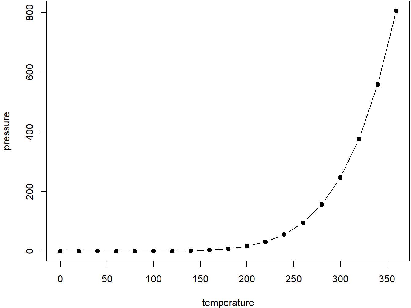
Figure 2.1: Here is a nice figure!
Reference a figure by its code chunk label with the fig: prefix, e.g., see Figure 2.1. Similarly, you can reference tables generated from knitr::kable(), e.g., see Table 2.1.
Code
knitr::kable(
  head(iris, 20), caption = 'Here is a nice table!',
  booktabs = TRUE
)| Sepal.Length | Sepal.Width | Petal.Length | Petal.Width | Species |
|---|---|---|---|---|
| 5.1 | 3.5 | 1.4 | 0.2 | setosa |
| 4.9 | 3.0 | 1.4 | 0.2 | setosa |
| 4.7 | 3.2 | 1.3 | 0.2 | setosa |
| 4.6 | 3.1 | 1.5 | 0.2 | setosa |
| 5.0 | 3.6 | 1.4 | 0.2 | setosa |
| 5.4 | 3.9 | 1.7 | 0.4 | setosa |
| 4.6 | 3.4 | 1.4 | 0.3 | setosa |
| 5.0 | 3.4 | 1.5 | 0.2 | setosa |
| 4.4 | 2.9 | 1.4 | 0.2 | setosa |
| 4.9 | 3.1 | 1.5 | 0.1 | setosa |
| 5.4 | 3.7 | 1.5 | 0.2 | setosa |
| 4.8 | 3.4 | 1.6 | 0.2 | setosa |
| 4.8 | 3.0 | 1.4 | 0.1 | setosa |
| 4.3 | 3.0 | 1.1 | 0.1 | setosa |
| 5.8 | 4.0 | 1.2 | 0.2 | setosa |
| 5.7 | 4.4 | 1.5 | 0.4 | setosa |
| 5.4 | 3.9 | 1.3 | 0.4 | setosa |
| 5.1 | 3.5 | 1.4 | 0.3 | setosa |
| 5.7 | 3.8 | 1.7 | 0.3 | setosa |
| 5.1 | 3.8 | 1.5 | 0.3 | setosa |
You can write citations, too. For example, we are using the bookdown package [@R-bookdown] in this sample book, which was built on top of R Markdown and knitr [@xie2015].
Finally, here is an example of an interactive plot that leverages HTML and Javascript we can use for illustrating statistical distributions. (These only work for HTML format and not LaTex nor PDF.)
This is an interactive table
Code
DT::datatable(iris)2.1 Interactive Plots
and here are a few examples of interactive plots using plotly and other packages. The R Graph Gallery is a good reference for the type of plots at our disposal.
Code
p <- gapminder %>%
  filter(year==1977) %>%
  ggplot( aes(gdpPercap, lifeExp, size = pop, color=continent)) +
  geom_point() +
  theme_bw()

ggplotly(p)
Code
theUrl <- "http://vincentarelbundock.github.io/Rdatasets/csv/reshape2/tips.csv"
tips <- read.table(file = theUrl, header = TRUE, sep = ",")

p <- ggplot(tips, aes(x=total_bill, weight = tip, color=sex, fill = sex)) +
  geom_histogram(binwidth=2.5) +
  ylab("sum of tip") +
  geom_rug(sides="t", length = unit(0.3, "cm"))
fig <- ggplotly(p)
fig
Code
df <- read.csv('https://raw.githubusercontent.com/plotly/datasets/master/iris-data.csv')

pl_colorscale=list(c(0.0, '#19d3f3'),
               c(0.333, '#19d3f3'),
               c(0.333, '#e763fa'),
               c(0.666, '#e763fa'),
               c(0.666, '#636efa'),
               c(1, '#636efa'))

axis = list(showline=FALSE,
            zeroline=FALSE,
            gridcolor='#ffff',
            ticklen=4)

fig <- df %>%
  plot_ly()
fig <- fig %>%
  add_trace(
    type = 'splom',
    dimensions = list(
      list(label='sepal length', values=~sepal.length),
      list(label='sepal width', values=~sepal.width),
      list(label='petal length', values=~petal.length),
      list(label='petal width', values=~petal.width)
    ),
    text=~class,
    marker = list(
      color = as.integer(df$class),
      colorscale = pl_colorscale,
      size = 7,
      line = list(
        width = 1,
        color = 'rgb(230,230,230)'
      )
    )
  )
## Warning in add_trace(., type = "splom", dimensions = list(list(label = "sepal length", : NAs
## introduced by coercionCode
fig <- fig %>%
  layout(
    title= 'Iris Data set',
    hovermode='closest',
    dragmode= 'select',
    plot_bgcolor='rgba(240,240,240, 0.95)',
    xaxis=list(domain=NULL, showline=F, zeroline=F, gridcolor='#ffff', ticklen=4),
    yaxis=list(domain=NULL, showline=F, zeroline=F, gridcolor='#ffff', ticklen=4),
    xaxis2=axis,
    xaxis3=axis,
    xaxis4=axis,
    yaxis2=axis,
    yaxis3=axis,
    yaxis4=axis
  )

fig