Chapter 3 Synchronous seminar
In this week of HE930, we will meet synchronously on Zoom to examine the predictive analytics process, discuss the ethics of using predictive analytics in HPEd, and apply predictive analytics together to a dataset.
Note that there is no assignment to complete and turn in this week. The only required work this week is to attend the synchronous seminar sessions on Zoom. Please try your best to attend these sessions. If you cannot attend, we will arrange for make-up activities for you to complete.
This week, our goals are to…
Engage in discussion about the application of predictive analytics to education.
Examine the ethical implications of using predictive analytics in health professions education, using examples from other fields.
Run a machine learning model in R and interpret the results in the context of educational analytics.
MOST IMPORTANTLY, please complete the following preparation before you attend the synchronous seminar sessions.
3.1 Preparation for synchronous seminar
Please watch the following two videos, which we will discuss in our synchronous seminar:
- “Predictive Analytics in Education: An introductory example”. https://youtu.be/wGE7C5w6hb4. Available on YouTube and also embedded below.
The slides for the video above are available at https://rpubs.com/anshulkumar/ClassificationExample2020.
The Social Dilemma on Netflix. This link might take you there: https://www.netflix.com/title/81254224. If you do not have access to this on your own, inform the course instructors and we will arrange for you to watch.
Finally, in addition to watching the two videos above, please review all Week 1 readings, if you have not done so already.
Once you complete the items above, you do not need to do anything else other than attending the scheduled synchronous sessions on Zoom.
3.2 Seminar details
The schedule for our synchronous meetings this week are below. You should have received invitations to your IHP email address to these sessions.
Important notes
- If you cannot attend any sessions, we will arrange a make-up activity (either a make-up meeting or an asynchronous activity).
- It is okay to arrive late or leave early from a session, if necessary. It is better to be there for some of each session than to miss it altogether.
Session 1: The Analytics Process.
- Time: Tuesday, May 27 2025, 1:00 – 3:00 p.m. US Eastern Time
- Location: Anshul’s Zoom room
To prepare for this session, please review all Week 1 readings and watch this 26-minute video: https://youtu.be/wGE7C5w6hb4.
Session 2: The Social Dilemma and Ethical Concerns of Machine Learning
- Time: Thursday, May 29 2025, 1:00 – 3:00 p.m. US Eastern Time
- Location: Anshul’s Zoom room
To prepare for this session, please watch The Social Dilemma on Netflix, which you can access at https://www.netflix.com/title/81254224.
Session 3: Machine Learning in R
- Time: Friday, May 30 2025, 2:00 – 4:00 p.m. US Eastern Time
- Location: Anshul’s Zoom room
During this session, we will do a machine learning tutorial in R and RStudio on our computers. Please be prepared to run RStudio on your computer and share your screen. No other preparation for this session is needed.
3.3 Session 1: The Analytics Process
3.3.1 Goal 1: Discuss the PA process and its applications
Reminder:
- PA = predictive analytics
- ML = machine learning
- PAML = predictive analytics and machine learning
- AI = artificial intelligence
This discussion will primarily be driven by questions and topics raised by students during the sessions itself. The items listed below are meant to supplement our discussion.
3.3.2 Questions & topics from weeks 1 & 2
3.3.2.1 Bias in prediction
- How do we make sure that predictive analytics doesn’t create bias, especially in small programs or teams like in a simulation center? For example, if we use data to decide which new educators are likely to succeed, how do we avoid reinforcing personal or cultural bias in the process? (AA)
3.3.3 Discussion questions from PA video/slides
How can predictive/learning analytics help you in your own work as an educator or at your organization/institution? What predictions would be useful for you to make?
How can you leverage data that your institution already collects (or that it is well-positioned to collect) using predictive analytic methods?
What would be the benefits and detriments of incorporating predictive analytics into your institution’s practices and processes?
Could predictive analysis complement any already-ongoing initiatives at your institution?
What would the ethical implications be of using predictive analytics at your institution? Would it cause unfair discrimination against particular learners? Would it help level the playing field for all learners?
3.3.4 Goal 2: Practice the PA process using simple examples (if time permits)
To achieve this goal, we will go through the Worksheet Packet used in the 2024 Quantitative Methods Workshop in the HE-942 seminar course. These are available in this week’s content module in D2L under the title “Worksheets for quantitative methods workshop from Anshul Kumar.”
3.3.5 Goal 3: Generate and discuss PA research questions (if time permits)
Discuss how PA can practically be used in HPEd and/or healthcare, especially in the settings in which we all work.
Generate research questions for using PA in HPEd.
Share and discuss answers to Task 16 in Week 1 discussions. Task 16: Find a case or example in the Ekowo & Palmer (2016) report that shows a way in which you wish that you could potentially use analytics within your own work or at your own institution. How is it (the case/example) similar to what you would like to do? How is it different?
3.4 Session 2: The Social Dilemma and Ethical Concerns of ML
3.4.1 Goals
Examine similarities and differences between social media analytics and HPEd analytics
Discuss ethics of predictive analytics
Practice predictive analytics research design (if time permits)
3.4.2 Discussion topics
Week 1 discussion questions related to ethics and PA/ML.
Will people start to behave differently just because they know that these models are being used to analyze them, subconsciously or consciously?
The same uses of predictive analytics shown in the movie, to make profit for the tech companies and for the people who advertise with detective companies, are also coming to Health Professions education at a very high speed. Are we ready for this?
Can we use the same technology to manipulate users for good purposes? Not only predict their outcomes but also cause them to do things to make their outcomes better? How appropriate or inappropriate is it for us to do this?
An interviewee in The Social Dilemma gave the example of Wikipedia showing different users different content based on what they were paid to show. As educators, we might show different materials to different students based on having analyzed their data. Is this the right or wrong thing to do? Who should control this capability? Should it even be possible or not?
How do the social media marketing frameworks on the previous slides relate to the relationships between people and technology in HPEd?


3.5 Session 3: Machine Learning in R
During this session, we will work together to complete and discuss the machine learning tutorial below.
3.5.1 Goals
Practice using decision tree and logistic regression models to predict which students are going to pass or fail, using the
student-por.csvdata.Fine-tune predictive models.
Compare the results of different predictive models and choose the best one.
Brainstorm about how the predictions would be used in an educational setting.
3.5.2 Important reminders
Anywhere you see the word
MODIFYis one place where you might consider making changes to the code.If you are not certain about any interpretations of results—especially confusion matrices, accuracy, sensitivity, and specificity—stop and ask an instructor for assistance.
For most of this tutorial, you will run the code below in an R script or R markdown file in RStudio on your own computer. You will also make minor modifications to this code.
3.5.3 Load relevant packages
Step 1: Load packages
if (!require(PerformanceAnalytics)) install.packages('PerformanceAnalytics') ## Warning: package 'xts' was built under R version 4.2.3## Warning: package 'zoo' was built under R version 4.2.3if (!require(rpart)) install.packages('rpart')
if (!require(rpart.plot)) install.packages('rpart.plot')
if (!require(car)) install.packages('car') ## Warning: package 'car' was built under R version 4.2.3if (!require(rattle)) install.packages('rattle') ## Warning: package 'tibble' was built under R version 4.2.3library(PerformanceAnalytics)
library(rpart)
library(rpart.plot)
library(car)
library(rattle)3.5.4 Import and describe data
We will use the student-por.csv data.
Step 2: Import data
d <- read.csv("student-por.csv")The best place to download this data is from D2L.
Data source and details:
P. Cortez and A. Silva. Using Data Mining to Predict Secondary School Student Performance. In A. Brito and J. Teixeira Eds., Proceedings of 5th FUture BUsiness TEChnology Conference (FUBUTEC 2008) pp. 5-12, Porto, Portugal, April, 2008, EUROSIS, ISBN 978-9077381-39-7. Available at https://archive.ics.uci.edu/ml/datasets/Student+Performance.
Alternate source: https://www.kaggle.com/larsen0966/student-performance-data-set
If the code above does not work to load the data, you can try this code instead:
d <- read.csv(file = "student-por.csv", sep = ";")Step 3: List variables
names(d)## [1] "school" "sex" "age" "address"
## [5] "famsize" "Pstatus" "Medu" "Fedu"
## [9] "Mjob" "Fjob" "reason" "guardian"
## [13] "traveltime" "studytime" "failures" "schoolsup"
## [17] "famsup" "paid" "activities" "nursery"
## [21] "higher" "internet" "romantic" "famrel"
## [25] "freetime" "goout" "Dalc" "Walc"
## [29] "health" "absences" "G1" "G2"
## [33] "G3"Description of dataset and all variables: https://archive.ics.uci.edu/ml/datasets/Student+Performance.
All variables in formula (for easy copying and pasting):
(b <- paste(names(d), collapse="+"))## [1] "school+sex+age+address+famsize+Pstatus+Medu+Fedu+Mjob+Fjob+reason+guardian+traveltime+studytime+failures+schoolsup+famsup+paid+activities+nursery+higher+internet+romantic+famrel+freetime+goout+Dalc+Walc+health+absences+G1+G2+G3"Step 4: Calculate number of observations
nrow(d)## [1] 649Step 5: Generate binary version of dependent variable, G3 (final grade, 0 to 20).
d$passed <- ifelse(d$G3 > 9.99, 1, 0)We’re assuming that a score of over 9.99 is a passing score, and below that is failing.
Step 6: Descriptive statistics for G3 continuous numeric variable.
summary(d$G3)## Min. 1st Qu. Median Mean 3rd Qu. Max.
## 0.00 10.00 12.00 11.91 14.00 19.00sd(d$G3)## [1] 3.230656Step 7: Who all passed and failed, binary qualitative categorical variable.
with(d, table(passed, useNA = "always"))## passed
## 0 1 <NA>
## 100 549 0Step 8: Histogram
hist(as.numeric(d$G3))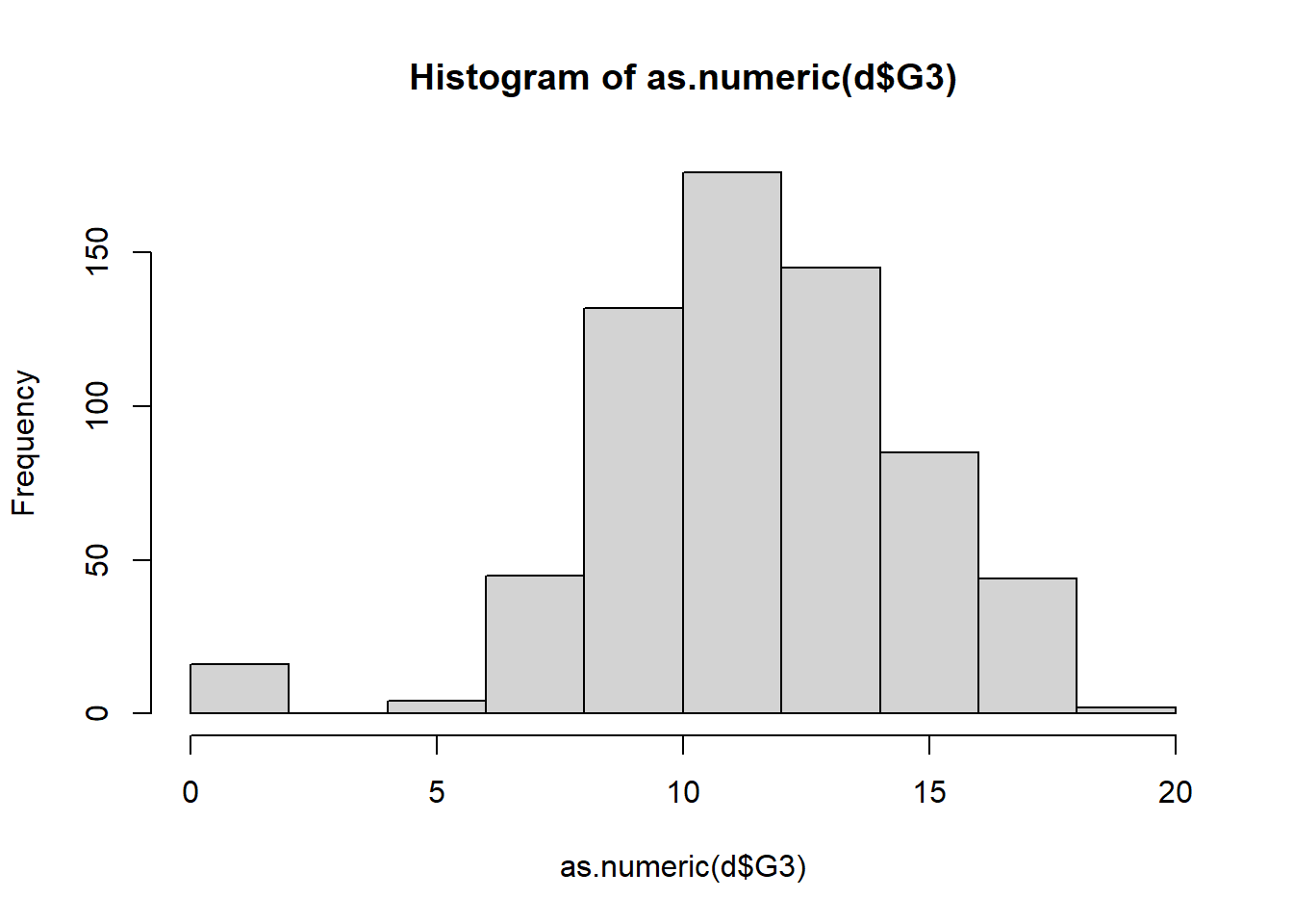
Step 9: Scatterplots
plot(d$G1 , d$G3) # MODIFY which variables you plot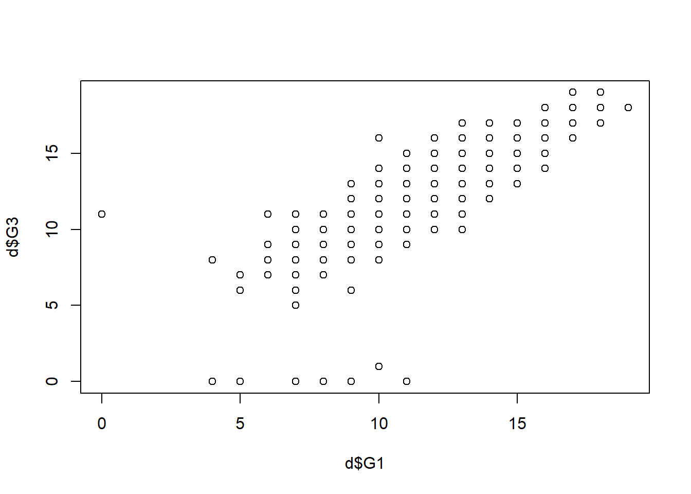
plot(d$health, d$G3)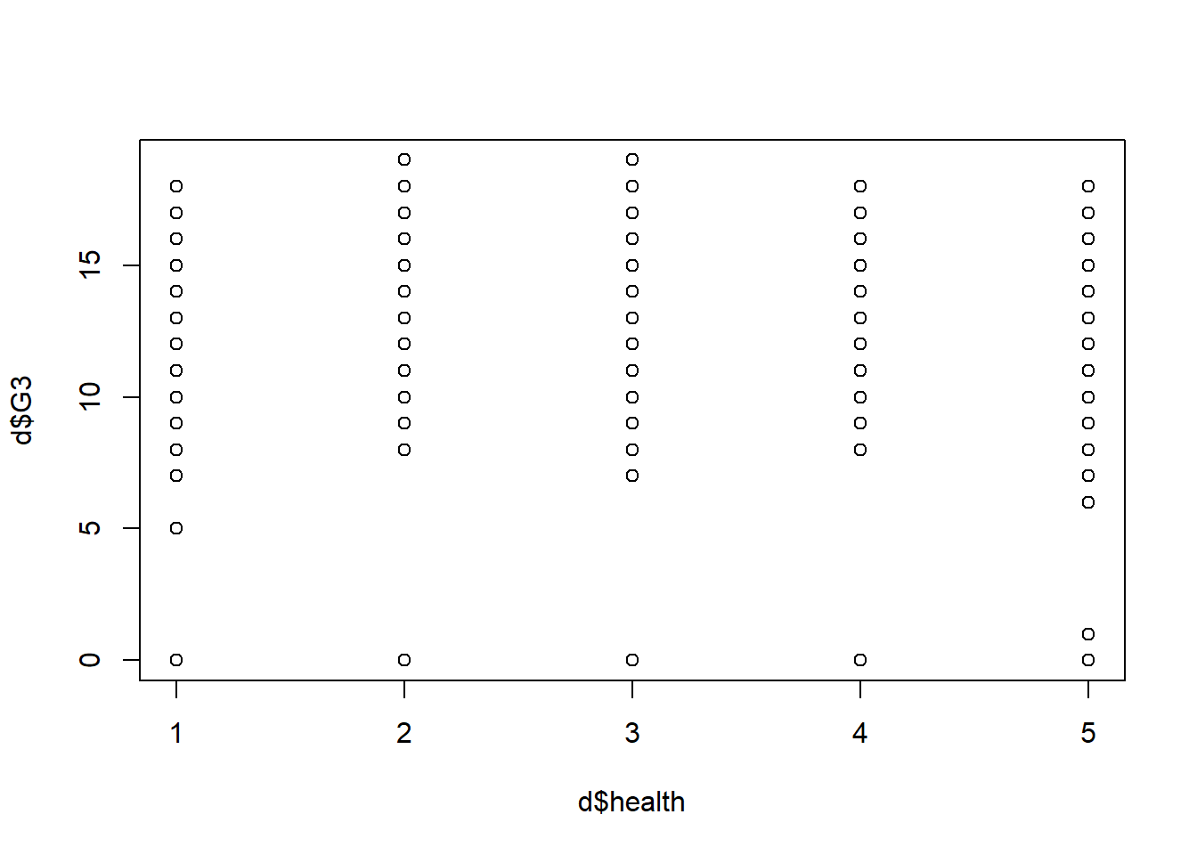
Step 10: Selected correlations (optional)
chart.Correlation(d[c("G3","G1","Medu","failures")], histogram=TRUE, pch=19) ## Warning in par(usr): argument 1 does not name a graphical parameter
## Warning in par(usr): argument 1 does not name a graphical parameter
## Warning in par(usr): argument 1 does not name a graphical parameter
## Warning in par(usr): argument 1 does not name a graphical parameter
## Warning in par(usr): argument 1 does not name a graphical parameter
## Warning in par(usr): argument 1 does not name a graphical parameter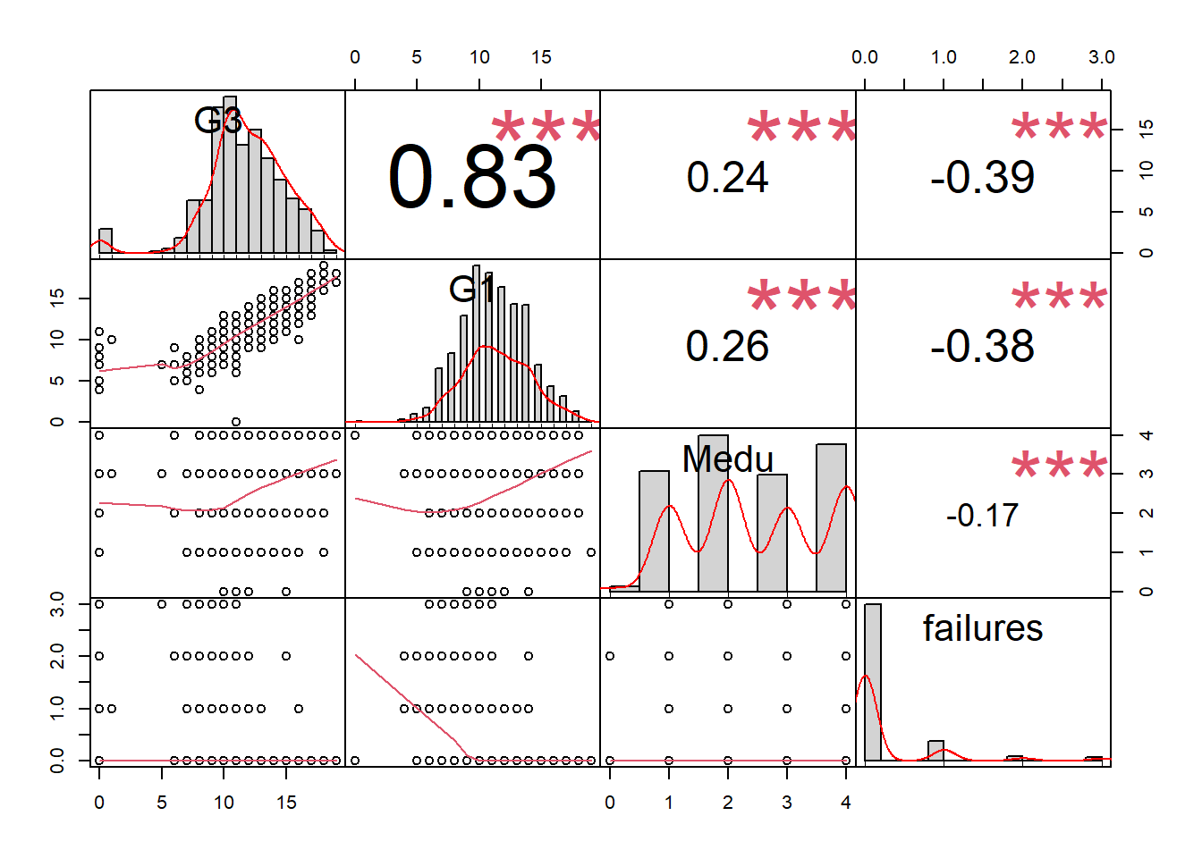
3.5.5 Divide training and testing data
Step 11: Divide data
trainingRowIndex <- sample(1:nrow(d), 0.75*nrow(d))  # row indices for training data
dtrain <- d[trainingRowIndex, ]  # model training data
dtest <- d[-trainingRowIndex, ] # test data3.5.6 Decision tree model – regression tree
Activity summary:
- Goal: predict continuous outcome
G3, using a regression tree. - Start by using all variables to make decision tree. Check predictive capability.
- Remove variables to make predictions with less information.
- Modify cutoff thresholds and see how confusion matrix changes.
- Anywhere you see the word
MODIFYis one place where you might consider making changes to the code. - Figure out which students to remediate.
3.5.6.1 Train and inspect model
Step 14: Train a decision tree model
tree1 <- rpart(G3 ~ school+sex+age+address+famsize+Pstatus+Medu+Fedu+Mjob+Fjob+reason+guardian+traveltime+studytime+failures+schoolsup+famsup+paid+activities+nursery+higher+internet+romantic+famrel+freetime+goout+Dalc+Walc+health+absences+G1+G2, data=dtrain, method = 'anova')
# MODIFY. Complete the next step (visualize the tree) and
# then come back to this and run the model without G1 and
# G2. Then try other combinations.

summary(tree1)
## Call:
## rpart(formula = G3 ~ school + sex + age + address + famsize +
## Pstatus + Medu + Fedu + Mjob + Fjob + reason + guardian +
## traveltime + studytime + failures + schoolsup + famsup +
## paid + activities + nursery + higher + internet + romantic +
## famrel + freetime + goout + Dalc + Walc + health + absences +
## G1 + G2, data = dtrain, method = "anova")
## n= 486
##
## CP nsplit rel error xerror xstd
## 1 0.53174438 0 1.0000000 1.0050672 0.10031853
## 2 0.13929193 1 0.4682556 0.4735021 0.06387449
## 3 0.09360831 2 0.3289637 0.3758442 0.04601341
## 4 0.05241337 3 0.2353554 0.2594922 0.03562257
## 5 0.01897086 4 0.1829420 0.2142600 0.03141879
## 6 0.01256090 5 0.1639712 0.1953945 0.03124297
## 7 0.01000000 6 0.1514103 0.1893802 0.03223584
##
## Variable importance
## G2 G1 school Medu failures Dalc absences
## 42 26 7 7 7 5 3
## Mjob famrel goout
## 1 1 1
##
## Node number 1: 486 observations, complexity param=0.5317444
## mean=12.02675, MSE=9.96842
## left son=2 (240 obs) right son=3 (246 obs)
## Primary splits:
## G2 < 11.5 to the left, improve=0.53174440, (0 missing)
## G1 < 11.5 to the left, improve=0.44866190, (0 missing)
## failures < 0.5 to the right, improve=0.17265670, (0 missing)
## higher splits as LR, improve=0.08380644, (0 missing)
## school splits as RL, improve=0.08375724, (0 missing)
## Surrogate splits:
## G1 < 11.5 to the left, agree=0.877, adj=0.750, (0 split)
## failures < 0.5 to the right, agree=0.626, adj=0.242, (0 split)
## school splits as RL, agree=0.623, adj=0.237, (0 split)
## Medu < 3.5 to the left, agree=0.611, adj=0.213, (0 split)
## Dalc < 1.5 to the right, agree=0.597, adj=0.183, (0 split)
##
## Node number 2: 240 observations, complexity param=0.1392919
## mean=9.695833, MSE=6.361649
## left son=4 (47 obs) right son=5 (193 obs)
## Primary splits:
## G2 < 8.5 to the left, improve=0.44198510, (0 missing)
## G1 < 8.5 to the left, improve=0.26816910, (0 missing)
## school splits as RL, improve=0.10506530, (0 missing)
## failures < 0.5 to the right, improve=0.09972261, (0 missing)
## absences < 0.5 to the left, improve=0.04307091, (0 missing)
## Surrogate splits:
## G1 < 7.5 to the left, agree=0.850, adj=0.234, (0 split)
## famrel < 1.5 to the left, agree=0.825, adj=0.106, (0 split)
##
## Node number 3: 246 observations, complexity param=0.09360831
## mean=14.30081, MSE=3.015203
## left son=6 (129 obs) right son=7 (117 obs)
## Primary splits:
## G2 < 13.5 to the left, improve=0.61140000, (0 missing)
## G1 < 14.5 to the left, improve=0.42049140, (0 missing)
## schoolsup splits as RL, improve=0.05237813, (0 missing)
## age < 16.5 to the left, improve=0.03977027, (0 missing)
## studytime < 1.5 to the left, improve=0.02961736, (0 missing)
## Surrogate splits:
## G1 < 13.5 to the left, agree=0.809, adj=0.598, (0 split)
## Medu < 3.5 to the left, agree=0.573, adj=0.103, (0 split)
## studytime < 2.5 to the left, agree=0.569, adj=0.094, (0 split)
## school splits as LR, agree=0.565, adj=0.085, (0 split)
## Mjob splits as LLLLR, agree=0.565, adj=0.085, (0 split)
##
## Node number 4: 47 observations, complexity param=0.05241337
## mean=6.297872, MSE=11.40063
## left son=8 (16 obs) right son=9 (31 obs)
## Primary splits:
## absences < 1 to the left, improve=0.4738903, (0 missing)
## G2 < 5.5 to the left, improve=0.3519696, (0 missing)
## health < 4.5 to the right, improve=0.1280191, (0 missing)
## reason splits as RRLL, improve=0.1280191, (0 missing)
## age < 17.5 to the right, improve=0.1107422, (0 missing)
## Surrogate splits:
## G2 < 2.5 to the left, agree=0.766, adj=0.313, (0 split)
## goout < 1.5 to the left, agree=0.723, adj=0.188, (0 split)
## Medu < 3.5 to the right, agree=0.702, adj=0.125, (0 split)
## Mjob splits as RRRRL, agree=0.702, adj=0.125, (0 split)
## schoolsup splits as RL, agree=0.702, adj=0.125, (0 split)
##
## Node number 5: 193 observations, complexity param=0.0125609
## mean=10.52332, MSE=1.638057
## left son=10 (115 obs) right son=11 (78 obs)
## Primary splits:
## G2 < 10.5 to the left, improve=0.19248510, (0 missing)
## G1 < 9.5 to the left, improve=0.14277070, (0 missing)
## failures < 0.5 to the right, improve=0.09399379, (0 missing)
## school splits as RL, improve=0.03543712, (0 missing)
## Mjob splits as LLLRR, improve=0.03407719, (0 missing)
## Surrogate splits:
## G1 < 9.5 to the left, agree=0.663, adj=0.167, (0 split)
## Mjob splits as LLLRL, agree=0.632, adj=0.090, (0 split)
## Medu < 3.5 to the left, agree=0.611, adj=0.038, (0 split)
## studytime < 2.5 to the left, agree=0.611, adj=0.038, (0 split)
## famrel < 2.5 to the right, agree=0.611, adj=0.038, (0 split)
##
## Node number 6: 129 observations
## mean=13.00775, MSE=0.7828856
##
## Node number 7: 117 observations, complexity param=0.01897086
## mean=15.7265, MSE=1.600409
## left son=14 (91 obs) right son=15 (26 obs)
## Primary splits:
## G2 < 16.5 to the left, improve=0.49083180, (0 missing)
## G1 < 16.5 to the left, improve=0.34527800, (0 missing)
## absences < 3.5 to the right, improve=0.05479733, (0 missing)
## Fjob splits as RRLRL, improve=0.03942344, (0 missing)
## reason splits as RLLR, improve=0.03707550, (0 missing)
## Surrogate splits:
## G1 < 16.5 to the left, agree=0.906, adj=0.577, (0 split)
##
## Node number 8: 16 observations
## mean=3.0625, MSE=15.80859
##
## Node number 9: 31 observations
## mean=7.967742, MSE=0.9344433
##
## Node number 10: 115 observations
## mean=10.06087, MSE=1.813686
##
## Node number 11: 78 observations
## mean=11.20513, MSE=0.5989481
##
## Node number 14: 91 observations
## mean=15.25275, MSE=0.9141408
##
## Node number 15: 26 observations
## mean=17.38462, MSE=0.46745563.5.6.2 Tree visualization
Step 15: Visualize decision tree model in two ways.
prp(tree1)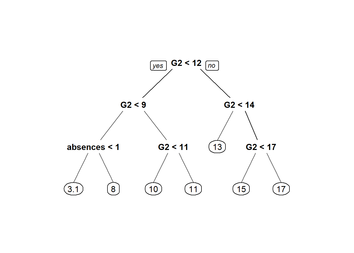
fancyRpartPlot(tree1, caption = "Regression Tree")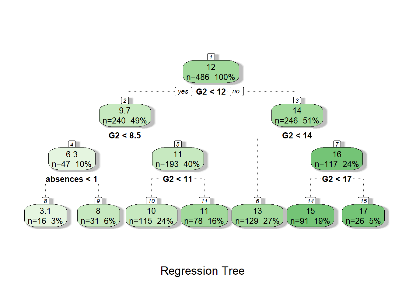
3.5.6.3 Test model
Step 16: Make predictions on testing data, using trained model
dtest$tree1.pred <- predict(tree1, newdata = dtest)Step 17: Visualize predictions
with(dtest, plot(tree1.pred, G3, main="Actual vs Predicted, testing data",xlab = "Actual G3",ylab = "Predicted G3"))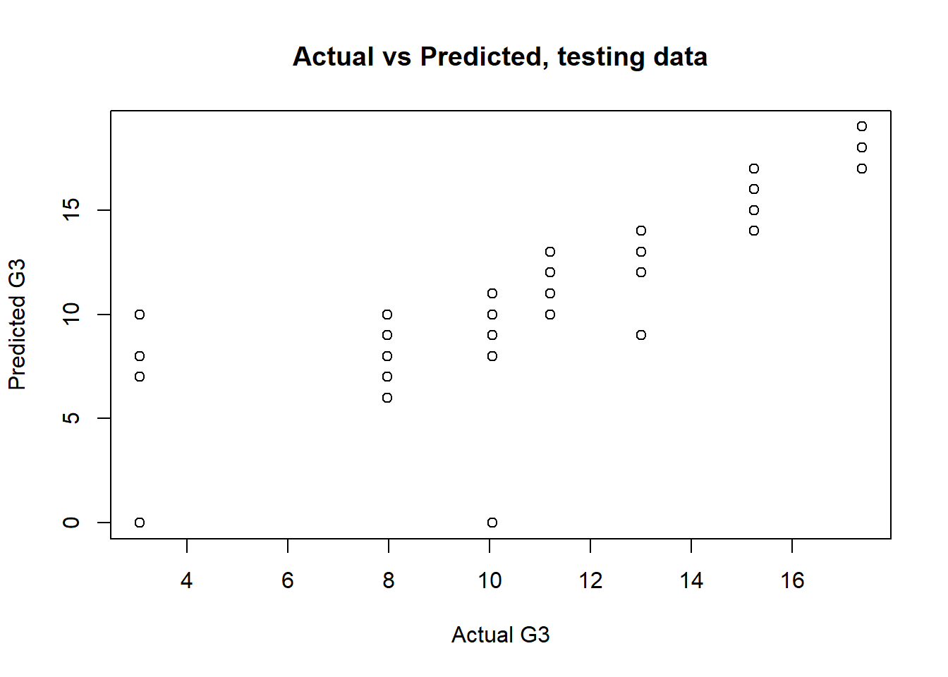
Step 18: Make confusion matrix.
PredictionCutoff <- 9.99 # MODIFY. Compare values in 9-11 range.

dtest$tree1.pred.passed <- ifelse(dtest$tree1.pred > PredictionCutoff, 1, 0)

(cm1 <- with(dtest,table(tree1.pred.passed,passed)))
## passed
## tree1.pred.passed 0 1
## 0 20 6
## 1 9 128Step 19: Calculate accuracy
CorrectPredictions1 <- cm1[1,1] + cm1[2,2]
TotalStudents1 <- nrow(dtest)

(Accuracy1 <- CorrectPredictions1/TotalStudents1)
## [1] 0.9079755Step 20: Sensitivity (proportion of people who actually failed that were correctly predicted to fail).
(Sensitivity1 <- cm1[1,1]/(cm1[1,1]+cm1[2,1]))## [1] 0.6896552Step 21: Specificity (proportion of people who actually passed that were correctly predicted to pass).
(Specificity1 <- cm1[2,2]/(cm1[1,2]+cm1[2,2]))## [1] 0.9552239BE SURE TO DOUBLE-CHECK THE CALCULATIONS ABOVE MANUALLY!
Step 22: It is very important for you, the data analyst, to modify the 9.99 cutoff assigned as PredictionCutoff above to see how you can change the predictions made by the model. Write down what you observe as you change this value and re-run the confusion matrix, accuracy, sensitivity, and specificity code above. What are the implications of your manual modification of this cutoff? Remind your instructors to discuss this, in case they forget!
3.5.7 Decision tree model – classification tree
Activity summary:
- Goal: predict binary outcome
passed, using a classification tree. - Start by using all variables to make decision tree. Check predictive capability.
- Remove variables to make predictions with less information.
- Modify cutoff thresholds and see how confusion matrix changes.
- Anywhere you see the word
MODIFYis one place where you might consider making changes to the code. - Figure out which students to remediate.
3.5.7.1 Train and inspect model
Step 23: Train a decision tree model
tree2 <- rpart(passed ~ school+sex+age+address+famsize+Pstatus+Medu+Fedu+Mjob+Fjob+reason+guardian+traveltime+studytime+failures+schoolsup+famsup+paid+activities+nursery+higher+internet+romantic+famrel+freetime+goout+Dalc+Walc+health+absences+G1+G2, data=dtrain, method = "class")
# MODIFY. Try without G1 and G2. Then try other combinations.

summary(tree2)
## Call:
## rpart(formula = passed ~ school + sex + age + address + famsize +
## Pstatus + Medu + Fedu + Mjob + Fjob + reason + guardian +
## traveltime + studytime + failures + schoolsup + famsup +
## paid + activities + nursery + higher + internet + romantic +
## famrel + freetime + goout + Dalc + Walc + health + absences +
## G1 + G2, data = dtrain, method = "class")
## n= 486
##
## CP nsplit rel error xerror xstd
## 1 0.63380282 0 1.0000000 1.0000000 0.10966720
## 2 0.02816901 1 0.3661972 0.3661972 0.06986974
## 3 0.01408451 4 0.2816901 0.4788732 0.07920128
## 4 0.01000000 5 0.2676056 0.4929577 0.08026862
##
## Variable importance
## G2 G1 Medu Mjob Walc Fedu famrel
## 60 21 3 3 2 2 1
## reason Dalc absences Fjob health freetime goout
## 1 1 1 1 1 1 1
##
## Node number 1: 486 observations, complexity param=0.6338028
## predicted class=1 expected loss=0.1460905 P(node) =1
## class counts: 71 415
## probabilities: 0.146 0.854
## left son=2 (47 obs) right son=3 (439 obs)
## Primary splits:
## G2 < 8.5 to the left, improve=72.145080, (0 missing)
## G1 < 8.5 to the left, improve=52.188580, (0 missing)
## failures < 0.5 to the right, improve=18.865450, (0 missing)
## school splits as RL, improve=13.799420, (0 missing)
## higher splits as LR, improve= 8.253517, (0 missing)
## Surrogate splits:
## G1 < 7.5 to the left, agree=0.926, adj=0.234, (0 split)
## famrel < 1.5 to the left, agree=0.905, adj=0.021, (0 split)
##
## Node number 2: 47 observations
## predicted class=0 expected loss=0.0212766 P(node) =0.09670782
## class counts: 46 1
## probabilities: 0.979 0.021
##
## Node number 3: 439 observations, complexity param=0.02816901
## predicted class=1 expected loss=0.05694761 P(node) =0.9032922
## class counts: 25 414
## probabilities: 0.057 0.943
## left son=6 (71 obs) right son=7 (368 obs)
## Primary splits:
## G1 < 9.5 to the left, improve=9.662111, (0 missing)
## G2 < 9.5 to the left, improve=7.232686, (0 missing)
## failures < 0.5 to the right, improve=2.052112, (0 missing)
## school splits as RL, improve=1.825062, (0 missing)
## freetime < 4.5 to the right, improve=1.350514, (0 missing)
## Surrogate splits:
## G2 < 9.5 to the left, agree=0.868, adj=0.183, (0 split)
## higher splits as LR, agree=0.847, adj=0.056, (0 split)
## failures < 0.5 to the right, agree=0.845, adj=0.042, (0 split)
## age < 20.5 to the right, agree=0.843, adj=0.028, (0 split)
##
## Node number 6: 71 observations, complexity param=0.02816901
## predicted class=1 expected loss=0.2957746 P(node) =0.1460905
## class counts: 21 50
## probabilities: 0.296 0.704
## left son=12 (35 obs) right son=13 (36 obs)
## Primary splits:
## Mjob splits as LLRLR, improve=2.434608, (0 missing)
## age < 15.5 to the left, improve=2.154514, (0 missing)
## absences < 6.5 to the right, improve=2.146512, (0 missing)
## G2 < 9.5 to the left, improve=2.035200, (0 missing)
## G1 < 8.5 to the left, improve=1.422016, (0 missing)
## Surrogate splits:
## Fjob splits as RRRLL, agree=0.662, adj=0.314, (0 split)
## health < 3.5 to the left, agree=0.662, adj=0.314, (0 split)
## freetime < 3.5 to the left, agree=0.648, adj=0.286, (0 split)
## goout < 4.5 to the left, agree=0.648, adj=0.286, (0 split)
## Walc < 3.5 to the left, agree=0.634, adj=0.257, (0 split)
##
## Node number 7: 368 observations
## predicted class=1 expected loss=0.01086957 P(node) =0.7572016
## class counts: 4 364
## probabilities: 0.011 0.989
##
## Node number 12: 35 observations, complexity param=0.02816901
## predicted class=1 expected loss=0.4285714 P(node) =0.07201646
## class counts: 15 20
## probabilities: 0.429 0.571
## left son=24 (14 obs) right son=25 (21 obs)
## Primary splits:
## Medu < 2.5 to the right, improve=3.809524, (0 missing)
## Fedu < 3.5 to the right, improve=3.214286, (0 missing)
## G2 < 9.5 to the left, improve=2.877123, (0 missing)
## Walc < 2.5 to the right, improve=2.877123, (0 missing)
## school splits as RL, improve=2.142857, (0 missing)
## Surrogate splits:
## Fedu < 3.5 to the right, agree=0.800, adj=0.500, (0 split)
## Mjob splits as RL-L-, agree=0.743, adj=0.357, (0 split)
## G2 < 9.5 to the left, agree=0.743, adj=0.357, (0 split)
## reason splits as RRLL, agree=0.714, adj=0.286, (0 split)
## absences < 3.5 to the right, agree=0.714, adj=0.286, (0 split)
##
## Node number 13: 36 observations
## predicted class=1 expected loss=0.1666667 P(node) =0.07407407
## class counts: 6 30
## probabilities: 0.167 0.833
##
## Node number 24: 14 observations
## predicted class=0 expected loss=0.2857143 P(node) =0.02880658
## class counts: 10 4
## probabilities: 0.714 0.286
##
## Node number 25: 21 observations, complexity param=0.01408451
## predicted class=1 expected loss=0.2380952 P(node) =0.04320988
## class counts: 5 16
## probabilities: 0.238 0.762
## left son=50 (7 obs) right son=51 (14 obs)
## Primary splits:
## Walc < 2.5 to the right, improve=2.3333330, (0 missing)
## school splits as RL, improve=1.7857140, (0 missing)
## absences < 1 to the left, improve=1.0008660, (0 missing)
## higher splits as LR, improve=0.7619048, (0 missing)
## Medu < 1.5 to the left, improve=0.7281385, (0 missing)
## Surrogate splits:
## Dalc < 1.5 to the right, agree=0.857, adj=0.571, (0 split)
## age < 15.5 to the left, agree=0.714, adj=0.143, (0 split)
## reason splits as RLR-, agree=0.714, adj=0.143, (0 split)
## paid splits as RL, agree=0.714, adj=0.143, (0 split)
##
## Node number 50: 7 observations
## predicted class=0 expected loss=0.4285714 P(node) =0.01440329
## class counts: 4 3
## probabilities: 0.571 0.429
##
## Node number 51: 14 observations
## predicted class=1 expected loss=0.07142857 P(node) =0.02880658
## class counts: 1 13
## probabilities: 0.071 0.9293.5.7.2 Tree Visualization
Step 24: Visualize decision tree model in two ways
prp(tree2)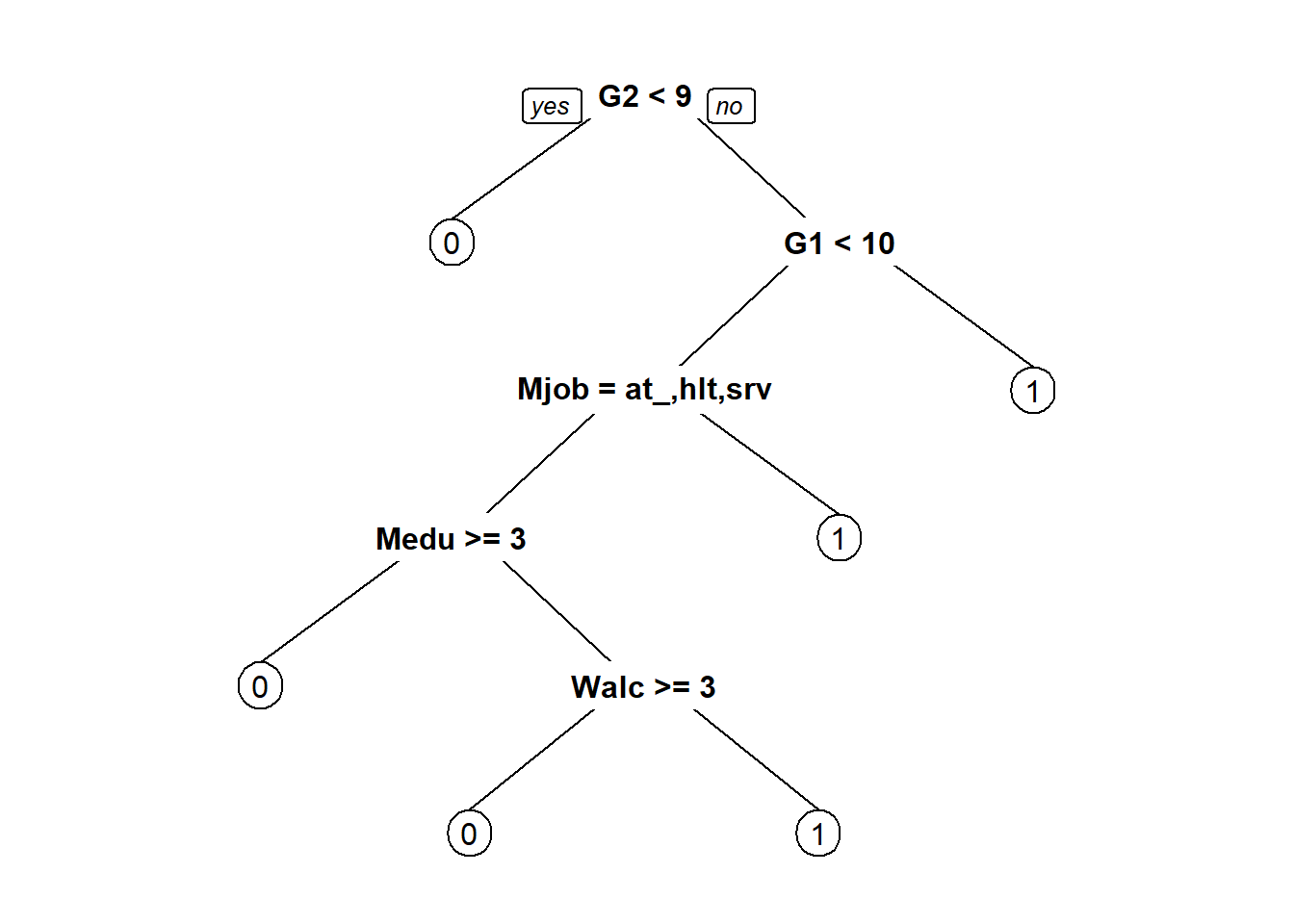
fancyRpartPlot(tree2, caption = "Classification Tree")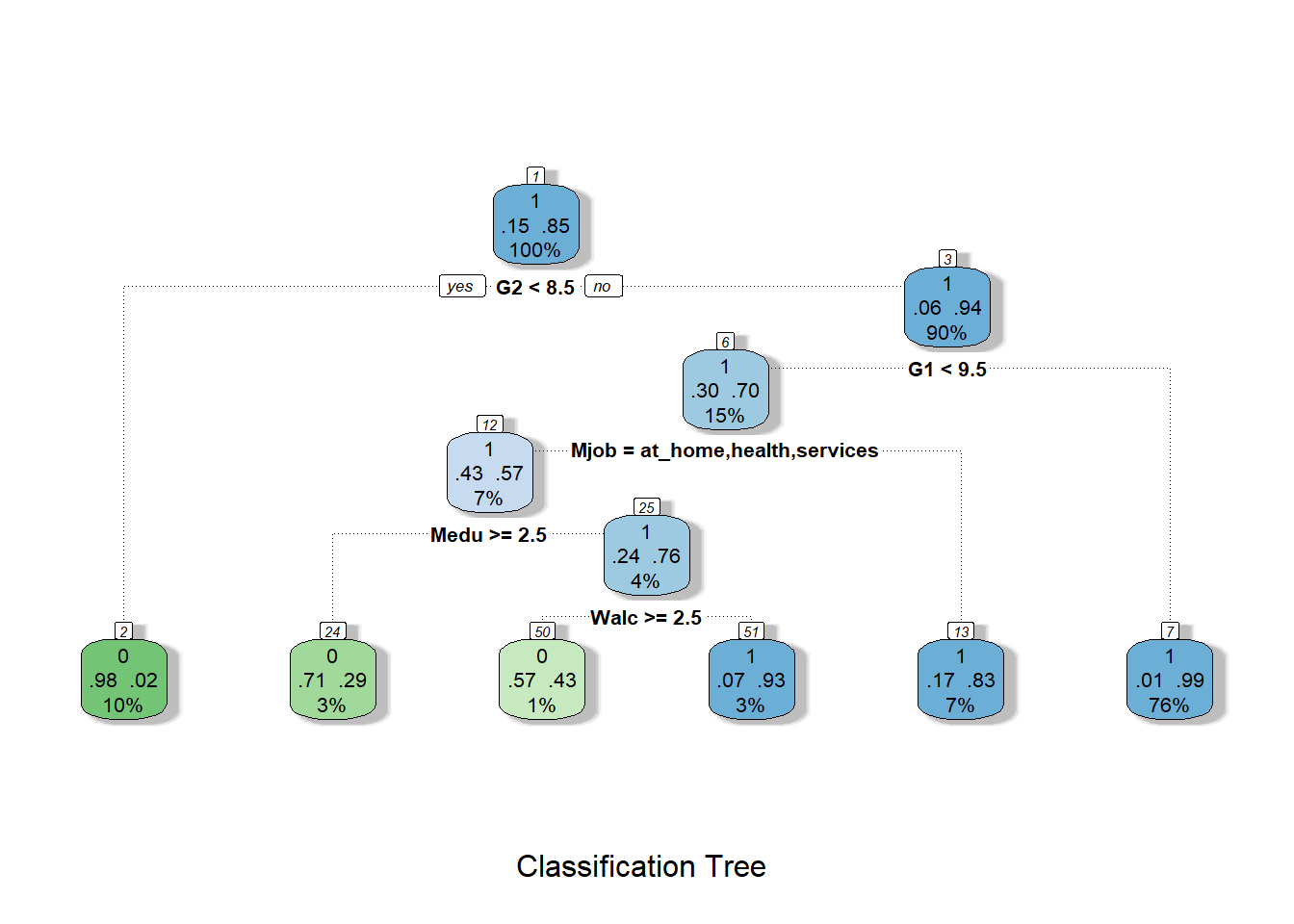
3.5.7.3 Test model
Step 25: Make predictions and confusion matrix on testing data classes, using trained model.
dtest$tree2.pred <- predict(tree2, newdata = dtest, type = 'class')
# MODIFY. change 'class' to 'prob'

(cm2 <- with(dtest,table(tree2.pred,passed)))
## passed
## tree2.pred 0 1
## 0 23 9
## 1 6 125Step 26: Make predictions and confusion matrix on testing data using probability cutoffs. Optional; results not shown.
dtest$tree2.pred <- predict(tree2, newdata = dtest, type = 'prob')

ProbabilityCutoff <- 0.5 # MODIFY. Compare different probability values.
dtest$tree2.pred.probs <- 1-dtest$tree2.pred[,1]

dtest$tree2.pred.passed <- ifelse(dtest$tree2.pred.probs > ProbabilityCutoff, 1, 0)

(cm2b <- with(dtest,table(tree2.pred.passed,passed)))
Step 27: Calculate accuracy
CorrectPredictions2 <- cm2[1,1] + cm2[2,2]
TotalStudents2 <- nrow(dtest)

(Accuracy2 <- CorrectPredictions2/TotalStudents2)
## [1] 0.9079755Step 28: Sensitivity (proportion of people who actually failed that were correctly predicted to fail)
(Sensitivity2 <- cm2[1,1]/(cm2[1,1]+cm2[2,1]))## [1] 0.7931034Step 29: Specificity (proportion of people who actually passed that were correctly predicted to pass):
(Specificity2 <- cm2[2,2]/(cm2[1,2]+cm2[2,2]))## [1] 0.9328358ALSO DOUBLE-CHECK THE CALCULATIONS ABOVE MANUALLY!
3.5.8 Logistic regression model – classification
Activity summary:
- Goal: predict binary outcome
passed, using logistic regression. - Start by using all variables to make a logistic regression model. Check predictive capability.
- Remove variables to make predictions with less information.
- Modify cutoff thresholds and see how confusion matrix changes.
- Anywhere you see the word
MODIFYis one place where you might consider making changes to the code. - Figure out which students to remediate.
3.5.8.1 Train and inspect model
Step 30: Train a logistic regression model
blr1 <- glm(passed ~ school+sex+age+address+famsize+Pstatus+Medu+Fedu+guardian+traveltime+studytime+failures+schoolsup+famsup+paid+activities+nursery+higher+internet+romantic+famrel+freetime+goout+Dalc+Walc+health+absences+Mjob+reason+Fjob+G1+G2, data=dtrain, family = "binomial")## Warning: glm.fit: fitted probabilities numerically 0 or 1 occurred# MODIFY. Try without G1 and G2. Then try other combinations.
# also remove variables causing multicollinearity and see if it makes a difference!
summary(blr1)##
## Call:
## glm(formula = passed ~ school + sex + age + address + famsize +
## Pstatus + Medu + Fedu + guardian + traveltime + studytime +
## failures + schoolsup + famsup + paid + activities + nursery +
## higher + internet + romantic + famrel + freetime + goout +
## Dalc + Walc + health + absences + Mjob + reason + Fjob +
## G1 + G2, family = "binomial", data = dtrain)
##
## Deviance Residuals:
## Min 1Q Median 3Q Max
## -2.37969 0.00000 0.00000 0.00048 2.30608
##
## Coefficients:
## Estimate Std. Error z value Pr(>|z|)
## (Intercept) -77.579708 22.865639 -3.393 0.000692 ***
## schoolMS -2.877074 1.424264 -2.020 0.043379 *
## sexM -0.616388 1.325614 -0.465 0.641943
## age 1.836987 0.665991 2.758 0.005811 **
## addressU 0.829745 1.108243 0.749 0.454036
## famsizeLE3 -0.204188 1.180564 -0.173 0.862685
## PstatusT -0.812378 1.995185 -0.407 0.683884
## Medu -0.281522 0.553640 -0.508 0.611107
## Fedu -0.438760 0.586167 -0.749 0.454144
## guardianmother -2.017849 1.477929 -1.365 0.172152
## guardianother 2.739071 2.357112 1.162 0.245217
## traveltime -0.431478 0.659120 -0.655 0.512708
## studytime 0.033363 0.701223 0.048 0.962053
## failures -1.599246 0.755478 -2.117 0.034271 *
## schoolsupyes -2.268786 1.712466 -1.325 0.185216
## famsupyes 0.433169 0.976196 0.444 0.657237
## paidyes -3.891068 2.403847 -1.619 0.105515
## activitiesyes 3.396239 1.412625 2.404 0.016208 *
## nurseryyes 1.337425 1.284950 1.041 0.297951
## higheryes -0.021735 1.101030 -0.020 0.984250
## internetyes -1.288519 1.361930 -0.946 0.344099
## romanticyes -3.975983 1.573985 -2.526 0.011535 *
## famrel -0.152447 0.494800 -0.308 0.758007
## freetime -0.966597 0.616195 -1.569 0.116728
## goout -0.620726 0.525726 -1.181 0.237721
## Dalc -0.266703 0.738870 -0.361 0.718129
## Walc 0.404973 0.747922 0.541 0.588188
## health -1.639290 0.796749 -2.057 0.039641 *
## absences -0.007599 0.105863 -0.072 0.942775
## Mjobhealth 4.908131 2.526967 1.942 0.052101 .
## Mjobother 3.302593 1.405972 2.349 0.018825 *
## Mjobservices 3.302204 2.200082 1.501 0.133370
## Mjobteacher 13.227145 5.392700 2.453 0.014175 *
## reasonhome -1.022717 1.645231 -0.622 0.534189
## reasonother -0.724290 1.698810 -0.426 0.669852
## reasonreputation -0.171650 1.711784 -0.100 0.920126
## Fjobhealth 6.425533 4.234905 1.517 0.129196
## Fjobother 0.958272 1.812836 0.529 0.597080
## Fjobservices -1.437612 1.935653 -0.743 0.457662
## Fjobteacher 22.060815 8.029470 2.747 0.006006 **
## G1 3.201345 1.026189 3.120 0.001811 **
## G2 3.829765 1.030249 3.717 0.000201 ***
## ---
## Signif. codes: 0 '***' 0.001 '**' 0.01 '*' 0.05 '.' 0.1 ' ' 1
##
## (Dispersion parameter for binomial family taken to be 1)
##
## Null deviance: 404.223 on 485 degrees of freedom
## Residual deviance: 66.693 on 444 degrees of freedom
## AIC: 150.69
##
## Number of Fisher Scoring iterations: 12car::vif(blr1)## GVIF Df GVIF^(1/(2*Df))
## school 4.744380 1 2.178160
## sex 4.615804 1 2.148442
## age 6.790783 1 2.605913
## address 3.214871 1 1.793006
## famsize 3.090062 1 1.757857
## Pstatus 3.364490 1 1.834255
## Medu 3.284670 1 1.812366
## Fedu 3.431544 1 1.852443
## guardian 11.546676 2 1.843377
## traveltime 2.905773 1 1.704633
## studytime 2.476413 1 1.573662
## failures 3.851065 1 1.962413
## schoolsup 3.339816 1 1.827516
## famsup 2.398073 1 1.548571
## paid 3.498089 1 1.870318
## activities 4.871489 1 2.207145
## nursery 2.567580 1 1.602367
## higher 2.178217 1 1.475878
## internet 4.594255 1 2.143421
## romantic 6.127876 1 2.475455
## famrel 2.533074 1 1.591563
## freetime 5.276808 1 2.297130
## goout 4.850766 1 2.202446
## Dalc 8.380783 1 2.894958
## Walc 10.904849 1 3.302249
## health 10.574686 1 3.251874
## absences 2.156020 1 1.468339
## Mjob 117.391408 4 1.814281
## reason 30.125383 3 1.763960
## Fjob 40.978317 4 1.590630
## G1 16.244707 1 4.030472
## G2 9.121276 1 3.0201453.5.8.2 Test model
Step 31: Make predictions on testing data, using trained model.
Predicting probabilities…
dtest$blr1.pred <- predict(blr1, newdata = dtest, type = 'response')

ProbabilityCutoff <- 0.5 # MODIFY. Compare different probability values.
dtest$blr1.pred.probs <- 1-dtest$blr1.pred

dtest$blr1.pred.passed <- ifelse(dtest$blr1.pred > ProbabilityCutoff, 1, 0)

(cm3 <- with(dtest,table(blr1.pred.passed,passed)))
## passed
## blr1.pred.passed 0 1
## 0 20 8
## 1 9 126Step 32: Make confusion matrix
(cm3 <- with(dtest,table(blr1.pred.passed,passed)))## passed
## blr1.pred.passed 0 1
## 0 20 8
## 1 9 126Step 33: Calculate accuracy
CorrectPredictions3 <- cm3[1,1] + cm3[2,2]
TotalStudents3 <- nrow(dtest)

(Accuracy3 <- CorrectPredictions3/TotalStudents3)
## [1] 0.8957055Step 34: Sensitivity (proportion of people who actually failed that were correctly predicted to fail)
(Sensitivity3 <- cm3[1,1]/(cm3[1,1]+cm3[2,1]))## [1] 0.6896552Step 35: Specificity (proportion of people who actually passed that were correctly predicted to pass)
(Specificity3 <- cm3[2,2]/(cm3[1,2]+cm3[2,2]))## [1] 0.9402985ALSO DOUBLE-CHECK THE CALCULATIONS ABOVE MANUALLY!
Step 36: It is very important for you, the data analyst, to modify the 0.5 cutoff assigned as ProbabilityCutoff above to see how you can change the predictions made by the model. Write down what you observe as you change this value and re-run the confusion matrix, accuracy, sensitivity, and specificity code above. What are the implications of your manual modification of this cutoff? Remind your instructors to discuss this, in case they forget!