1 Basic R

Learning Objectives:

This chapter covers common basic R functions used for statistical analysis. After finishing this chapter, you should be able to:

Define R variables.
Know the differences between an atomic variable and an object variable.
Perform arithmetic operators.
Store results in variables.
Format and print the contents of variables to the console.
Calculate non-robust and robust statistics.
Use seq() and with() functions.

As R scripting is a hands-on topic, I encourage you to open RStudio alongside this book and try out the code to maximize understanding. Let’s get started.

1.1 Rules of Naming Variables

The name of an R variable must follow these two rules:

It must begin with a letter (A-Z or a-z), a dot “.”, or an underscore “_”, and
Subsequent characters can be any combinations of letters, digits (0-9), “.”, or “_”.

Note that:

Variable names are case-sensitive, e.g., volume and Volume are different in the eyes of R.
Give meaningful names to variables, e.g., zone2 instead of z or even worse x. That will help a bunch in understanding the code, even your own code.
Watch out that some names have been used by R, e.g., c, and head are function names. However, R is permissive for people to use them as variable names. So, the rule of thumb is to exercise self-discipline not to choose R function names as variable names.

1.2 R Objects

1.2.1 Atomic and Object Variables

R classifies variables into two broad categories: atomic variables, and objects. In the former, the value cannot be split further into smaller R objects. E.g., the height of an object is 5.6 feet:

height <- 5.6

In mathematics, an atomic variable is a scalar.

On the other hand, an R object comprises different components that can be accessed individually or split into other R objects. E.g.,

# A simple numeric vector for the days in each month
days_of_month <- c(31, 28, 31, 30, 31, 30, 31, 31, 30, 31, 30, 31)

days_of_month is a vector object in R. c() is the collate function, as its name suggests, it combines or packs a list of values into a vector object. You can extract the days of a month like:

# Days in February
print(days_of_month[2])
#> [1] 28

[2] means the 2^nd element of a vector. We will discuss more about indexing below. vector is only one of the many types of objects supported by R, more object types will be discussed later.

1.2.2 Numeric variables

R’s numeric data type includes whole numbers, decimal numbers, and numbers represented in scientific notation ($6.023e^{23}$). Here are some examples:

# Decimal
height <- 5.6

# Whole number (Integer)
sample_size <- 15

# Scientific notation
avogadro_number <- 6.023e23

Don’t be mistaken, the e in the scientific notation refers to base 10, e.g., 6.023e23 is $6.023x10^{23}$.

<- denotes the assignment operator. Upon execution, the resultant value of the expression on the right-hand side, if no error, is stored in the named variable on the left-hand side. In RStudio, you can see the variable name and its associated value under the Environment tab, which usually occupies the top right quadrant.

Note that R supports two equivalent assignment operators. You can use <- and = interchangeably. I prefer <- to = as = can easily confuse with the equality checking operator ==.

1.2.3 Arithmetic Operators

Arithmetic operators include +, -, *, /, **, and ^. The last two operators - ** and ^ - are exponential; they perform exactly the same function. Here are some examples:

radius <- 2.5
diameter <- 2*pi*radius
area <- pi*radius**2
volume <- (4/3)*pi*radius^3

Note that pi is $\pi$, which is a built-in variable with the value 3.141593.

1.2.3.1 Printing and Formatting

R provides a function called print() that prints text to the console. E.g.,

print("Hello World!")
#> [1] "Hello World!"

radius <- 2.5
diameter <- 2*pi*radius
print(diameter)
#> [1] 15.70796

Suppose you want to improve the printout by making it more readable, say "The diameter of a circle with radius 2.5 cm is 15.70796." In such a case, you need the format function paste(). Here’s how to use it:

radius <- 2.5
diameter <- 2*pi*radius
print(paste("The diameter of a circle with radius",radius,"cm is",diameter,"."))
#> [1] "The diameter of a circle with radius 2.5 cm is 15.707963267949 ."

The above printout is almost perfect. If you’re picky, you don’t like the extra space separating the diameter and the period in the above message, you can use paste()’s cousin function paste0(). The difference between the two is that paste0() will not automatically add an extra space between each component given to the function. Below is the previous print statement with paste0():

print(paste0("The diameter of a circle with radius",radius,"cm is",diameter,"."))
#> [1] "The diameter of a circle with radius2.5cm is15.707963267949."

As you can see, there is no more space between the diameter and the period. But it created other issues; there is no space between “The diameter of a circle with radius” and the actual radius as well. So, when you use paste0(), you have to take care of the space separation yourselves. Here is the final version for using paste0():

print(paste0("The diameter of a circle with radius ",radius," cm is ",diameter,"."))
#> [1] "The diameter of a circle with radius 2.5 cm is 15.707963267949."

1.2.4 Character variables

You can store non-numeric values in variables by embracing the character value with a pair of quotes, either a pair of single or double quotes. E.g.,

course <- 'BIOL265'
nucleotides <- c('A','C','G','T')

To figure out whether a variable’s type is numeric, character, or something else, use the class() function,

class(course)
#> [1] "character"

class(days_of_month)
#> [1] "numeric"

Obviously, it does not make sense to do math with character type. E.g.,

nucleotides*4
#> Error in nucleotides * 4: non-numeric argument to binary operator

1.2.5 Factors/Categorical Variables

In R, a categorical variable in statistics is called a factor. A categorical variable is further split into nominal or ordinal. A nominal variable has no intrinsic order. Use the factor() function to define a factor. E.g., a sample of colors is stored in a vector, and you want to define it as a categorical variable.

colors <- c("Red","Blue","Blue","Red","Green","Green","Blue","Green","Red","Blue")
colors <- factor(colors, levels=c('Red','Blue','Green'))
print(colors)
#>  [1] Red   Blue  Blue  Red   Green Green Blue  Green Red  
#> [10] Blue 
#> Levels: Red Blue Green

Categorical variables with intrinsic order are called ordinal variables. E.g.,

patients <- c("Stage 2","Hyperintensive","Stage 2","Hyperintensive","elevated","Stage 2","elevated","Stage 1")
patients <- factor(patients, levels=c('normal','elevated','Stage 1','Stage 2','Hyperintensive'),ordered = TRUE)
print(patients)
#> [1] Stage 2        Hyperintensive Stage 2       
#> [4] Hyperintensive elevated       Stage 2       
#> [7] elevated       Stage 1       
#> 5 Levels: normal < elevated < Stage 1 < ... < Hyperintensive

1.2.6 Data frames

Besides vector, another commonly used object is data frame. Almost. all the datasets we will use for analysis are in a data frame format. Simply speaking, a data frame is a tabular or spreadsheet-like object, like an Excel or Google Sheets. A data frame consists of rows and columns. Each row represents a sample. Each column represents a variable. Rows are expected to have equal length, i.e., the same number of columns. If not, R will either complain or pad the missing columns with a special value NA (not available). Let’s take a look at an R’s built-in data frame iris:

# Show the first five rows
head(iris)
#>   Sepal.Length Sepal.Width Petal.Length Petal.Width Species
#> 1          5.1         3.5          1.4         0.2  setosa
#> 2          4.9         3.0          1.4         0.2  setosa
#> 3          4.7         3.2          1.3         0.2  setosa
#> 4          4.6         3.1          1.5         0.2  setosa
#> 5          5.0         3.6          1.4         0.2  setosa
#> 6          5.4         3.9          1.7         0.4  setosa

You can peek into the bottom five rows by the tail() function.

tail(iris)
#>     Sepal.Length Sepal.Width Petal.Length Petal.Width
#> 145          6.7         3.3          5.7         2.5
#> 146          6.7         3.0          5.2         2.3
#> 147          6.3         2.5          5.0         1.9
#> 148          6.5         3.0          5.2         2.0
#> 149          6.2         3.4          5.4         2.3
#> 150          5.9         3.0          5.1         1.8
#>       Species
#> 145 virginica
#> 146 virginica
#> 147 virginica
#> 148 virginica
#> 149 virginica
#> 150 virginica

As you can see, the data frame consists of five variables (columns). Here are the R functions to show the shape of a data frame:

# the dimension (row x column) of a data frame.
dim(iris)
#> [1] 150   5

# Only the number of rows
nrow(iris)
#> [1] 150

# Only the number of columns
ncol(iris)
#> [1] 5

So, we know that iris contains 150 rows (flowers) and five columns.

1.2.6.1 Accessing Rows and Columns of a Data Frame

Each element in a data frame can be referenced by row and column indexes like the X-Y Cartesian system. Rows are automatically indexed (numbered), where the 1st row is index 1, the 2nd row is index 2, and the index of the last row is the total number of rows, similarly for columns. But often time, columns are named, such as the columns of iris; Sepal.Width, Sepal.Length, etc., as shown in Figure (1.1). The two equivalent indexing schemes can occur in parallel.¹

The syntax of accessing individual elements is <data frame name>[row, column]. E.g., the cell at the 5^th row and 3^rd column of the iris is:

iris[5,3]
#> [1] 1.4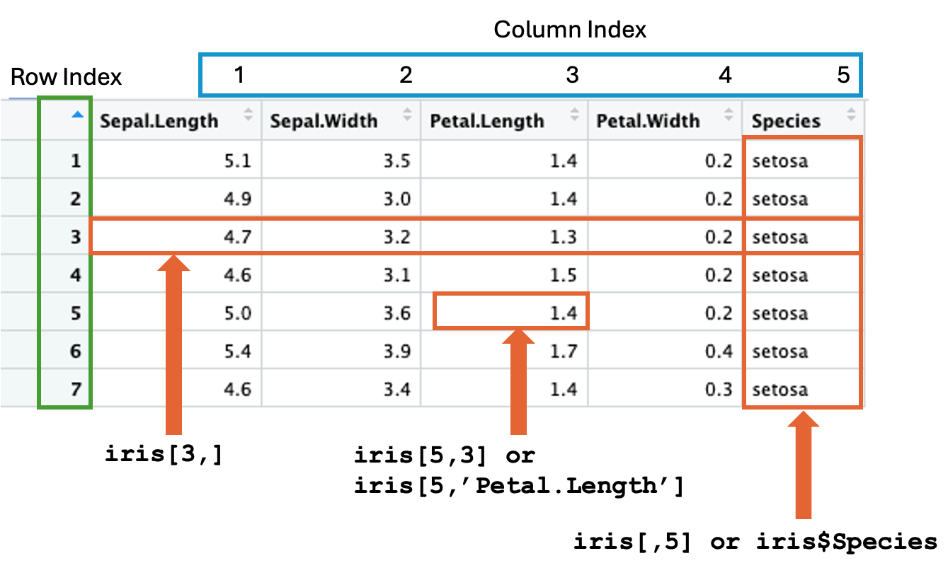

Figure 1.1: Accessing rows and columns of a data frame.

If the column index is ignored, all columns of the specified row(s) are returned as shown in Figure (1.1). For example, show all columns of the 3^rd row by:

# Specify the row number only and leave out the column index.
iris[3,]
#>   Sepal.Length Sepal.Width Petal.Length Petal.Width Species
#> 3          4.7         3.2          1.3         0.2  setosa

Similarly, if the row index is skipped, all rows of the specified column(s) are returned (1.1). For example,

# Specify only the column index.
head(iris[,5])
#> [1] setosa setosa setosa setosa setosa setosa
#> Levels: setosa versicolor virginica

R provides an alternative way to access a single column of a data frame. The syntax is <data frame name>$<column name>. The equivalence of iris[,5] is iris$Species:

head(iris$Species)
#> [1] setosa setosa setosa setosa setosa setosa
#> Levels: setosa versicolor virginica

Note that the $ method only works for a single column. We will discuss a way shortly how to access multiple columns in one R command.

Besides the numeric column index, columns can be referenced by names as shown in Figure (1.1). E.g., the Petal.Length of the 5^th row:

iris[5,'Petal.Length']
#> [1] 1.4

To access more than one column and row, pack the row indices and column names in vectors by the collate function (c(...)). For example, show the Petal.Length and Sepal.Length of the 123^th and 96^th rows:

iris[c(123,96),c('Petal.Length','Sepal.Length')]
#>     Petal.Length Sepal.Length
#> 123          6.7          7.7
#> 96           4.2          5.7

Using row index and column names is the basic accessing method. R provides additional methods to select rows and columns by conditions. More of this topic will be discussed in Chapter 2: Data Wrangling.

1.2.7 Descriptive Statistics

1.2.7.1 Summary Functions

length() shows the number elements in an object. We will use a sample of pumpkin’s weights for illustration.

# A sample of pumpkins' weights
pumpkins <- c(6.85,6.56,6.23,7.55,4.45,10.14,3.52,6.62,3.76,7.62)

The length() shows the number of weights defined in pumpkins.

length(pumpkins)
#> [1] 10

To be clear, length() counts the number of elements in an R object, such as a vector or a data frame. If the object is atomic, the function will return 1. For example, in the following example, dna is a character (atomic). The function will return 1, not the number of characters.

dna <- 'ACGTAGC'
length(dna)
#> [1] 1

The range() prints the minimum and maximum values - numeric and non-numeric - of an object.

range(pumpkins)
#> [1]  3.52 10.14

If you are interested in either the minimum or maximum, here are the corresponding functions:

# The lightness
min(pumpkins)
#> [1] 3.52

# The heaviest
max(pumpkins)
#> [1] 10.14

1.2.7.2 Non-robust Statistics

Mean, variance, and standard deviation are non-robust statistics, as they are sensitive to outliers (extreme values).

# A sample of pumpkins' weights
pumpkins <- c(6.85,6.56,6.23,7.55,4.45,10.14,3.52,6.62,3.76,7.62)

# The average weight
mean(pumpkins)
#> [1] 6.33

# The variance
var(pumpkins)
#> [1] 4.013489

# the standard deviation
sd(pumpkins)
#> [1] 2.003369

1.2.7.3 Robust Statistics

Median and quantile are robust statistics, as outliers minimally influence their values.

Median

# A sample of pumpkins' weights
pumpkins <- c(6.85,6.56,6.23,7.55,4.45,10.14,3.52,6.62,3.76,7.62)

median(pumpkins)
#> [1] 6.59

Quantile

Standard quantile intervals.

quantile(pumpkins)
#>     0%    25%    50%    75%   100% 
#>  3.520  4.895  6.590  7.375 10.140

A customized quantile intervals.

quantile(pumpkins, probs = c(0.1,0.9))
#>   10%   90% 
#> 3.736 7.872

A specific quantile.

quantile(pumpkins, probs = c(0.05))
#>    5% 
#> 3.628

quantile(pumpkins, probs = c(0.95))
#>   95% 
#> 9.006

Inter-quantile Region (IQR)

\[IQR = Q3 - Q1\]

IQR(pumpkins)
#> [1] 2.48

1.2.7.4 `summary()` Function

A data frame may consists of many variables of different types in various ranges. Therefore, it makes a lot of sense to take a glimpse of all variables before analysis. It can be done by the summary() function to reveal:

The variable type of each column.
If the column is numeric, a summary of numeric values.
If the column is categorical (factor), what are the levels and order, if it is ordinal.

Let’s see the summary of iris:

summary(iris)
#>   Sepal.Length    Sepal.Width     Petal.Length  
#>  Min.   :4.300   Min.   :2.000   Min.   :1.000  
#>  1st Qu.:5.100   1st Qu.:2.800   1st Qu.:1.600  
#>  Median :5.800   Median :3.000   Median :4.350  
#>  Mean   :5.843   Mean   :3.057   Mean   :3.758  
#>  3rd Qu.:6.400   3rd Qu.:3.300   3rd Qu.:5.100  
#>  Max.   :7.900   Max.   :4.400   Max.   :6.900  
#>   Petal.Width          Species  
#>  Min.   :0.100   setosa    :50  
#>  1st Qu.:0.300   versicolor:50  
#>  Median :1.300   virginica :50  
#>  Mean   :1.199                  
#>  3rd Qu.:1.800                  
#>  Max.   :2.500

The summary will show the range (min. and max.) and quantiles of a numeric column. For a categorical variable (factor), it will show the levels with the number of samples (rows) found for each level, e.g., Species is a nominal variable, with 50 samples per species.

1.3 Utilities

1.3.1 `seq()` - create a series of numbers

There are situations where we need a series of equal-interval numbers. For example, override the default breaks - x-ticks - of a histogram, a vector containing all possible outcomes of tossing two dice, i.e, from 2 to 12.

In R, the seq() function generates a list of equal-interval numbers, whole and decimal. seq() takes the following parameters:

from = 1, the default is 1.
to = 1, the default is 1.
by = 1, the size of the interval between two adjacent numbers. It takes integer and decimal numbers. If it is negative, the series is decreasing.
length.out specifies how many numbers are returned. This option is an alternative to by when you care only about how many numbers are generated instead of the interval between them. See the example below.
along.with, it generates the same number of numbers according to what is provided to the along.with parameter.

Examples

By default, seq() begins with 1 and has an interval of 1. E.g., generate 10 integers starting with 1.

seq(10)
#>  [1]  1  2  3  4  5  6  7  8  9 10

Staring from and ending with.

seq(-10,10)
#>  [1] -10  -9  -8  -7  -6  -5  -4  -3  -2  -1   0   1   2   3
#> [15]   4   5   6   7   8   9  10

Specify the interval.

seq(-10,10, by=2)
#>  [1] -10  -8  -6  -4  -2   0   2   4   6   8  10

A decreasing sequence.

seq(10,by=-1)
#>  [1] 10  9  8  7  6  5  4  3  2  1

Just specify the desired numbers to be generated. As you can see, the interval is pretty precise.

seq(-5,7,length.out=20)
#>  [1] -5.00000000 -4.36842105 -3.73684211 -3.10526316
#>  [5] -2.47368421 -1.84210526 -1.21052632 -0.57894737
#>  [9]  0.05263158  0.68421053  1.31578947  1.94736842
#> [13]  2.57894737  3.21052632  3.84210526  4.47368421
#> [17]  5.10526316  5.73684211  6.36842105  7.00000000

Generate a sequence that matches the same number in another sequence.

x <- seq(1,5)
cat("x =",x,"\n")
#> x = 1 2 3 4 5
y <- seq(-5, along.with=x)
cat("y =",y,"\n")
#> y = -5 -4 -3 -2 -1

Note: What is the difference between cat(...) and print(paste(...)) you saw above? The main difference is that print(paste(...)) creates an R object (a text) and then prints it, while cat(...) directly writes text to the console without creating a formal R object. See example below you will understand the nuance.

msg1 <- print(paste("Hello","World"))
#> [1] "Hello World"
print(msg1)
#> [1] "Hello World"

msg2 <- cat("Hello","World","\n")
#> Hello World
print(msg2)
#> NULL

Is it really important? No, unless you’re a R developer.

1.3.2 `with()`

It set up the context of a data frame so it spares you from using the $ to access the columns of a data frame. It is commonly used together with a function applied to one or more columns. E.g., the median of Petal.Width. It can done in two ways:

# Use $
median(iris$Petal.Width)
#> [1] 1.3

# Or, use with()
with(iris, median(Petal.Width))
#> [1] 1.3

For the straightforward example above, you do not see the value of with(). Let’s consider a more complicated row selection example. Find Sepal.Length in iris where its Petal.Length is less than 4 and Petal.Width is greater than 1. The $-way is:

iris$Sepal.Length[iris$Petal.Length<4 & iris$Petal.Width>1]
#> [1] 5.2 5.6 5.6 5.5 5.8 5.1

Here’s the with() version that saves typing iris repeatedly.

with(iris, Sepal.Length[Petal.Length<4 & Petal.Width>1])
#> [1] 5.2 5.6 5.6 5.5 5.8 5.1

In short, with() is English, so it improves the readability of R statements. Second, it saves some typing of the data frame’s name. I recommend using with() whenever possible.

1.4 Summary

That’s a bare minimum of R scripting required for data analysis. In the next chapter, we will focus on operations applied to data frames. Before you leave, it is useful to recap the R functions discussed in this chapter:

<-, c(), print(), paste(), paste0(), cat(), class(), factor(), head(), tail(), dim(), nrow(), ncol(), summary(), mean(), var(), sd(), range(), min(), max(), median(), quantile(), IQR(), seq(), and with().

Part I

2 Data Wrangling