5 Limits of Functions
In the previous chapter Operations on Functions, we explored how to combine functions through addition, subtraction, multiplication, division, and composition. These operations allowed us to model multi-step processes and represent interactions between different mathematical and real-world quantities.
In this chapter (See, Figure 5.1), we extend that understanding by studying Limits of Functions, which analyze the behavior of functions as their inputs approach specific points or infinity. Limits are a fundamental concept in calculus, forming the foundation for continuity, derivatives, and integrals. They allow us to rigorously describe how functions behave near critical points, handle discontinuities, and model phenomena where changes are instantaneous or unbounded.
5.1 Review
Before diving into formal definitions, let’s use an analogy to understand what a limit is. Imagine you are driving a car toward a stop sign. As you get closer, your speed gradually decreases, approaching zero. You never jump from a high speed to zero instantly—the approach is smooth and continuous. Similarly, in mathematics, a limit describes the value a function is approaching as the input gets closer to a particular point, even if the function doesn’t exactly reach that value at the point itself.
This animation (Figure 5.2) illustrates this concept by showing a car approaching a stop sign over time. The distance to the stop sign is represented by the function \(d(t) = 10 e^{-0.3 t}\), which decreases exponentially, approaching zero as time increases. The visualization highlights how the car’s distance diminishes gradually, making the idea of a limit intuitive and easy to grasp.
Explanation of the Graph: \((d(t) = 10 e^{-0.3 t}\)
The graph (Figure 5.2) illustrates the concept of a mathematical limit, showing how the car’s distance to a stop sign decreases over time and approaches zero without ever becoming negative.
- Blue line: shows the car’s distance to the stop sign over time.
- Blue point: represents the car’s position at each moment, moving down along the function.
- Red dashed line: the stop sign, acting as a horizontal asymptote at \(y = 0\).
- Function behavior:
- Exponentially decreasing: the distance drops quickly at first, then gradually approaches zero.
- Always decreasing → the car never moves away from the stop sign.
- Exponentially decreasing: the distance drops quickly at first, then gradually approaches zero.
- Limit: \(\lim_{t \to \infty} d(t) = 0\) → the car approaches the stop sign but never passes it.
5.2 Basic Limits
The limit of a function describes the behavior of the function as the input approaches a particular point. Formally, the limit of a function \(f(x)\) as \(x \to a\) is written as:
\[ \lim_{x \to a} f(x) = L \]
This means that as \(x\) gets closer to \(a\), \(f(x)\) gets closer to \(L\).
Example: \[ f(x) = 2x + 3 \] \[ \lim_{x \to 1} f(x) = 2(1) + 3 = 5 \]
Notes:
- The limit does not have to equal the function’s value at that point.
- If \(f(a)\) exists, the limit may equal \(f(a)\). If not, the limit can still exist.
5.3 Evaluation Techniques
In calculus, understanding how to evaluate limits is essential for analyzing the behavior of functions near specific points or as they approach infinity. Various techniques are used to simplify complex expressions, handle indeterminate forms, and determine whether a limit exists or diverges. These methods form the foundation for deeper topics such as continuity, derivatives, and integrals.
The following section presents several key techniques commonly used in evaluating limits, including direct substitution, factoring, rationalization, simplifying complex fractions, and applying special limit theorems. Each technique helps to reveal the underlying structure of a function and ensures accurate computation of limits in different contexts.
5.3.1 Direct Substitution
If \(f(x)\) is continuous at \(x = a\), then:
\[ \lim_{x \to a} f(x) = f(a) \]
Example: \[ \lim_{x \to 2} (3x + 1) = 3(2) + 1 = 7 \]
5.3.2 Factoring and Simplifying
Used when substitution gives an indeterminate form \(0/0\).
Example: \[ \lim_{x \to 2} \frac{x^2 - 4}{x - 2} \]
Factor the numerator:
\[ \frac{(x - 2)(x + 2)}{x - 2} \]
Cancel \((x - 2)\), then substitute:
\[ \lim_{x \to 2} (x + 2) = 4 \]
5.3.3 Rationalizing
Rationalizing (Conjugate Method) used when square roots cause indeterminate forms.
Example:
\[ \lim_{x \to 0} \frac{\sqrt{x + 4} - 2}{x} \]
Multiply by the conjugate: \[ \frac{\sqrt{x + 4} - 2}{x} \cdot \frac{\sqrt{x + 4} + 2}{\sqrt{x + 4} + 2} = \frac{x}{x(\sqrt{x + 4} + 2)} = \frac{1}{\sqrt{x + 4} + 2} \]
Then substitute \(x = 0\):
\[ \lim_{x \to 0} \frac{1}{\sqrt{4} + 2} = \frac{1}{4} \]
5.3.4 Dividing by the Highest Power of \(x\)
Used for limits at infinity with rational functions.
Example: \[ \lim_{x \to \infty} \frac{3x^2 + 2}{x^2 + 5} \]
Divide numerator and denominator by \(x^2\):
\[ \frac{3 + \frac{2}{x^2}}{1 + \frac{5}{x^2}} \to \frac{3}{1} = 3 \]
5.3.5 L’Hôpital’s Rule
Used for indeterminate forms \(\frac{0}{0}\) or \(\frac{\infty}{\infty}\). If \(\displaystyle \lim_{x \to a} \frac{f(x)}{g(x)}\) gives \(\frac{0}{0}\) or \(\frac{\infty}{\infty}\), then:
\[ \lim_{x \to a} \frac{f(x)}{g(x)} = \lim_{x \to a} \frac{f'(x)}{g'(x)} \] Example:
\[ \lim_{x \to 1} \frac{x^2 - 1}{x - 1} \]
At $x = 14:
\[ \frac{1^2 - 1}{1 - 1} = \frac{0}{0} \] This expression results in an indeterminate form, meaning the limit cannot be directly evaluated by simple substitution.
Therefore, differentiate numerator and denominator: \[ \frac{d}{dx}(x^2 - 1) = 2x, \quad \frac{d}{dx}(x - 1) = 1 \]
Then: \[ \lim_{x \to 1} \frac{2x}{1} = 2 \]
5.4 Special Limits
Special limits are common patterns that appear frequently in calculus. They often involve trigonometric, exponential, or logarithmic functions that have well-known limit results. Understanding these helps simplify many limit problems quickly.
5.4.1 Trigonometric Limit
\(\lim_{x \to 0} \frac{\sin x}{x}\)
This is one of the most fundamental limits in calculus.
\[ \lim_{x \to 0} \frac{\sin x}{x} = 1 \]
Reasoning:
As \(x\) approaches 0, both \(\sin x\) and \(x\) approach 0 at the same rate. Graphically, the sine curve and the line \(y = x\) are nearly identical near the origin.
Variants: \[ \lim_{x \to 0} \frac{\tan x}{x} = 1, \quad \lim_{x \to 0} \frac{1 - \cos x}{x} = 0 \]
5.4.2 Exponential Limit
\(\displaystyle \lim_{x \to 0} (1 + x)^{1/x}\)
This limit defines the mathematical constant \(e\) (Euler’s number).
\[ \lim_{x \to 0} (1 + x)^{1/x} = e \]
Alternative form:
\[ \lim_{n \to \infty} \left(1 + \frac{1}{n}\right)^{n} = e \]
Interpretation: This expression arises naturally in compound interest and growth models, it represents continuous growth where compounding occurs infinitely often.
5.4.3 Exponential Functions
For any real number \(k\):
\[ \lim_{x \to 0} e^{kx} = 1 \] since \(e^{kx} \to e^0 = 1\).
5.4.4 Logarithmic Functions
\[ \lim_{x \to 0^+} \ln(1 + x) = 0, \quad \lim_{x \to \infty} \frac{\ln x}{x} = 0 \]
5.4.5 Trigonometric Functions
\[ \lim_{x \to 0} \frac{\sin(kx)}{x} = k, \quad \lim_{x \to 0} \frac{1 - \cos(kx)}{x^2} = \frac{k^2}{2} \]
5.5 Discontinuities
5.5.1 One-Sided Limits
Left-hand limit (approaching from the left):
\[
\lim_{x \to a^-} f(x) = L
\]
The function approaches \(L\) as \(x\) approaches \(a\) from the left (\(x < a\)).
Right-hand limit (approaching from the right):
\[
\lim_{x \to a^+} f(x) = L
\]
The function approaches \(L\) as \(x\) approaches \(a\) from the right (\(x > a\)).
Limit exists if:
\[
\lim_{x \to a^-} f(x) = \lim_{x \to a^+} f(x)
\]
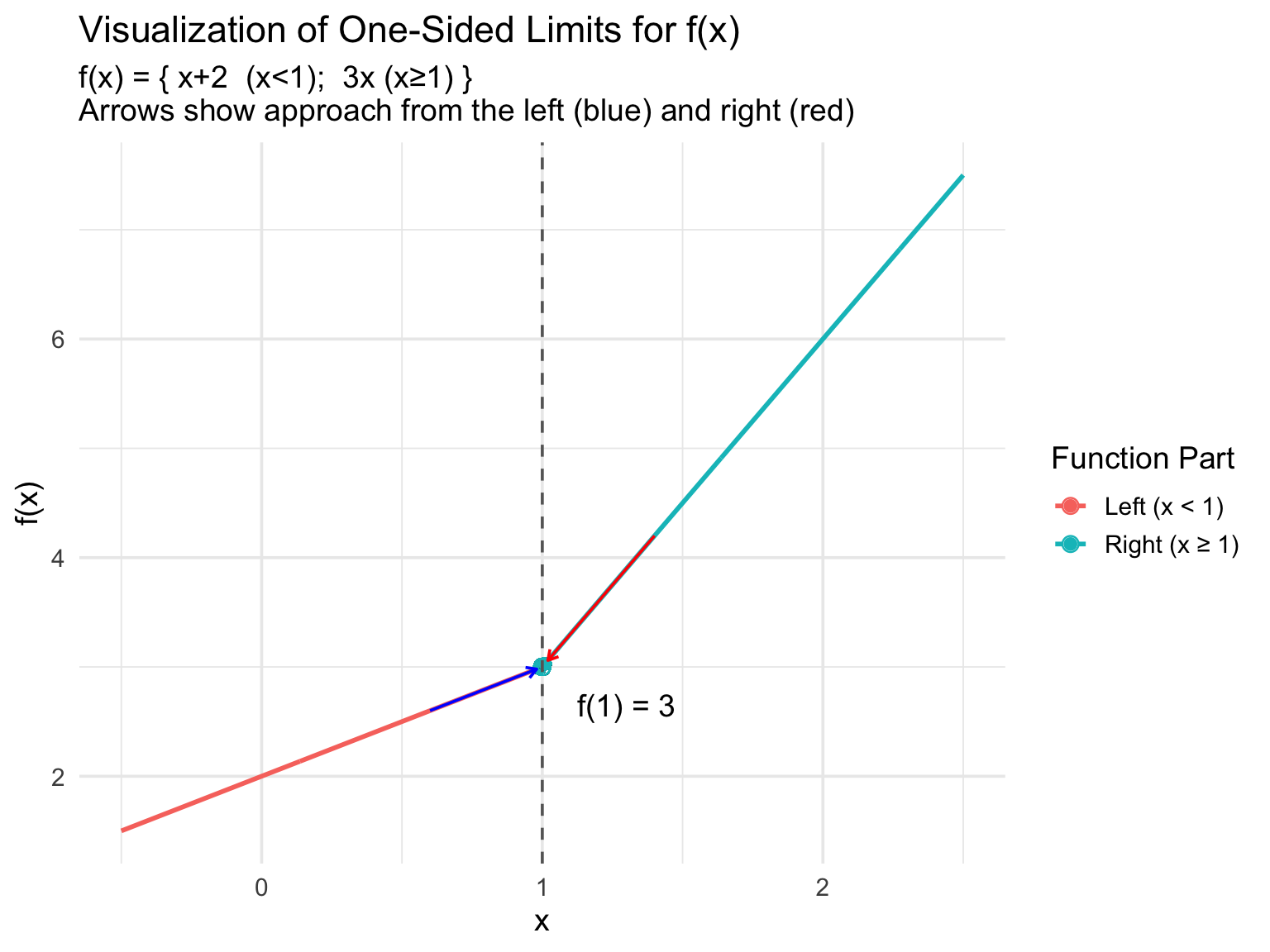
Example: \[ f(x) = \begin{cases} x + 2 & x < 1 \\ 3x & x \ge 1 \end{cases} \]
- \(\lim_{x \to 1^-} f(x) = 1 + 2 = 3\)
- \(\lim_{x \to 1^+} f(x) = 3(1) = 3\)
- So, \(\lim_{x \to 1} f(x) = 3\)
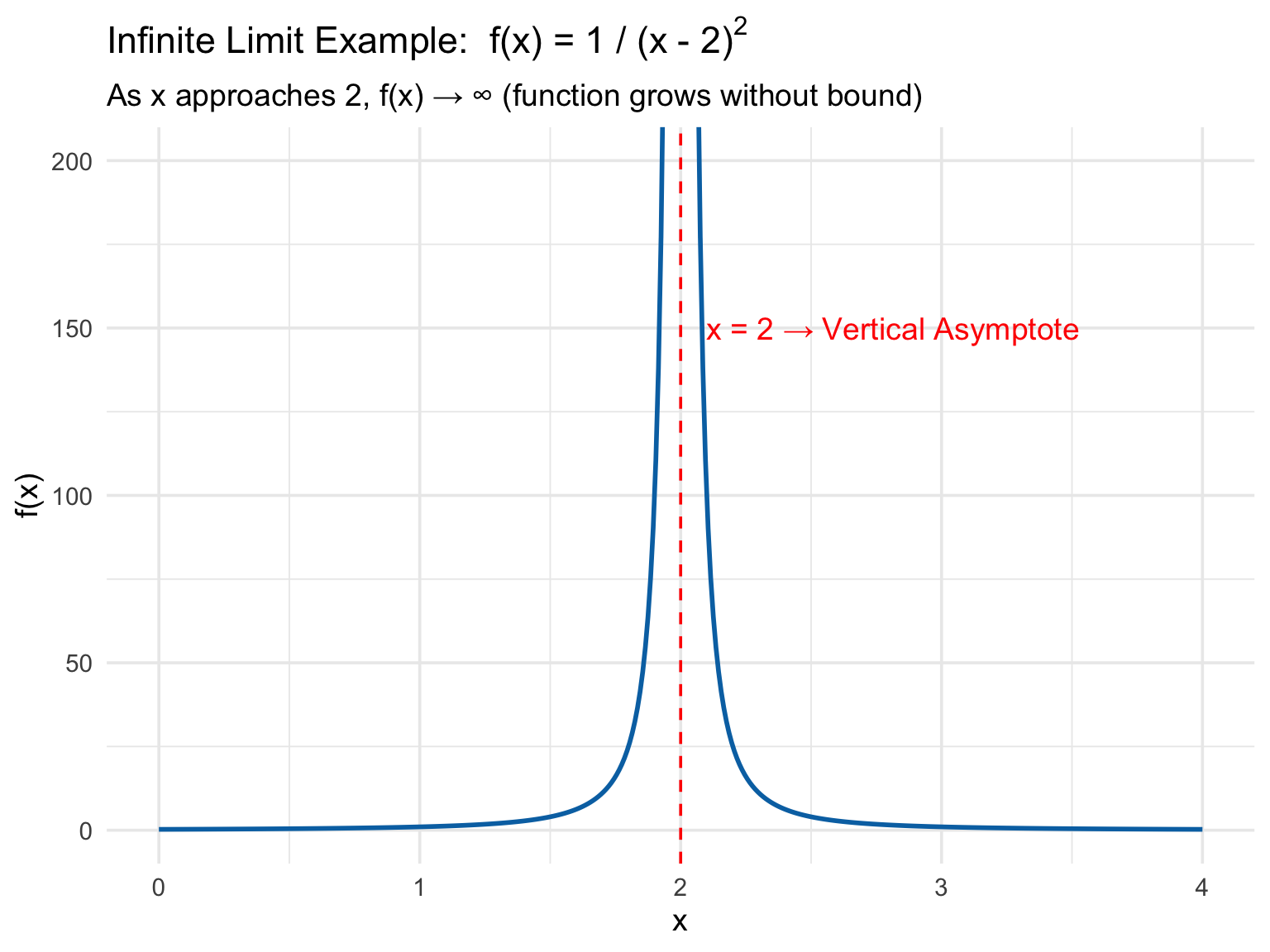
5.5.2 Infinite Limits
Infinite Limits (Vertical Asymptote) occur when the function grows without bound as it approaches a certain point. We are asking: “What happens to \(f(x)\) as \(x\) gets close to some point \(a\)?”
\[ \lim_{x \to a} f(x) = \infty \quad \text{or} \quad -\infty \]
Example: \[
f(x) = \frac{1}{(x-2)^2}
\]
\[
\lim_{x \to 2} f(x) = \infty
\]
This shows the function blows up as \(x\) approaches 2.
5.5.3 Limits at Infinity
These describe the end behavior of a function as \(x\) becomes very large (\(x \to \infty\)) or very small (\(x \to -\infty\)). We are asking: “What value does \(f(x)\) approach as \(x\) goes to infinity?”
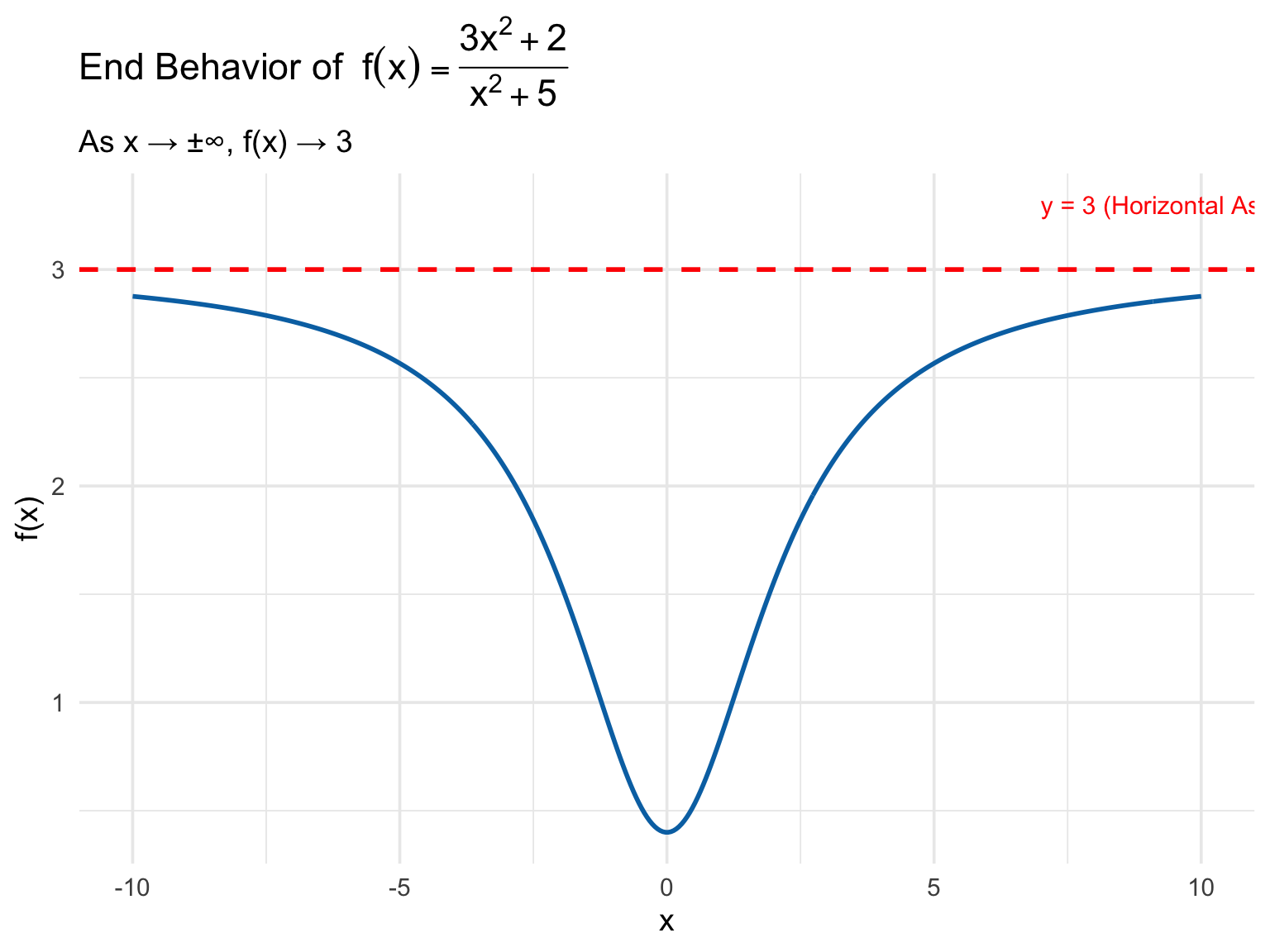
Consider the function:
\[ f(x) = \frac{3x^2 + 2}{x^2 + 5} \]
The degree of the numerator \(= 2\), and the degree of the denominator \(= 2\). \(\Rightarrow\) The degrees are the same. Take the coefficients of the highest-degree terms: Numerator \(= 3\), Denominator \(= 1\).
Therefore:
\[ \lim_{x \to \infty} f(x) = \frac{3}{1} = 3 \]
Step-by-step calculation (dividing by \(x^2\)):
\[ \frac{3x^2 + 2}{x^2 + 5} = \frac{3 + \frac{2}{x^2}}{1 + \frac{5}{x^2}} \]
As \(x \to \infty\), every term containing \(\frac{1}{x^2}\) approaches \(0\). Thus, we are left with:
\[ \frac{3}{1} = 3 \]
For \(x \to -\infty\): The same logic applies, since \(\frac{2}{x^2} \to 0\) and \(\frac{5}{x^2} \to 0\).
Therefore:
\[ \lim_{x \to -\infty} f(x) = 3 \]
*Conclusion: The graph of the function has a horizontal asymptote** at \(y = 3\) in both directions.
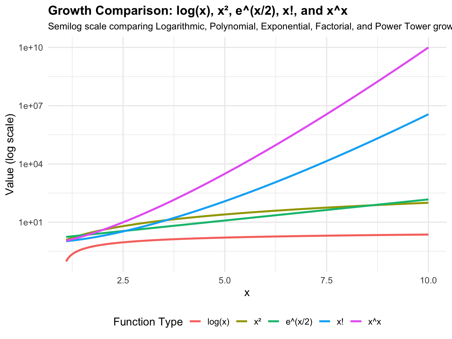
5.5.4 Growth Comparison
As \(x \to \infty\), some functions grow much faster than others. Understanding growth comparison is essential to:
- Evaluate limits at infinity,
- Identify horizontal asymptotes, and
- Determine which function dominates in complex expressions.
In general, the order of growth from slowest to fastest is:
\[ \ln(x) \ll x^a \ll a^x \ll x! \ll x^x \]
or verbally: Logarithmic < Polynomial < Exponential < Factorial < Power Tower
| Function Type | Example | Growth as \(x \to \infty\) | Notes |
|---|---|---|---|
| Logarithmic | \(\ln(x)\) | Slowest growth | Increases unboundedly but very slowly |
| Polynomial | \(x^2, x^3, x^n\) | Moderate growth | Dominates logarithmic functions |
| Exponential | \(2^x, e^x, 10^x\) | Fast growth | Always beats any polynomial |
| Factorial | \(x!\) | Very fast | Super-exponential growth |
| Power Tower | \(x^x, a^{x^2}\) | Extremely fast | Grows faster than all others |
5.6 Applications
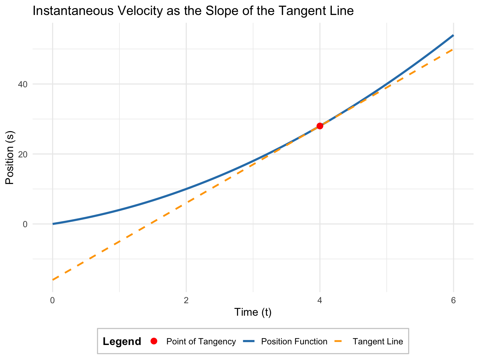
The concept of instantaneous velocity comes directly from the derivative of a function — a core application of limits and differential calculus. Suppose the position of an object moving along a straight line is given by a function:
\[ s = f(t) \]
where:
- \(s\) = position (in meters, for example)
- \(t\) = time (in seconds)
The average velocity of the object between two points in time \(t\) and \(t + h\) is defined as the change in position divided by the change in time:
\[ v_{\text{avg}} = \frac{\text{change in position}}{\text{change in time}} = \frac{f(t + h) - f(t)}{h} \]
This formula represents the average rate of change of the function \(f(t)\) over the interval \([t, t + h]\).
- If \(h\) is large, \(v_{\text{avg}}\) gives only a coarse estimate of the object’s motion.
- If \(h\) is small, \(v_{\text{avg}}\) becomes a more accurate approximation of how fast the object is moving at time \(t\).
To find the exact velocity at a single instant, we let the time interval \(h\) approach zero. This leads to the limit definition of the derivative:
\[ v(t) = \lim_{h \to 0} \frac{f(t + h) - f(t)}{h} \]
Thus, instantaneous velocity is defined as the derivative of the position function:
\[ v(t) = f'(t) \]
Geometrically, the expression
\[ \frac{f(t + h) - f(t)}{h} \]
represents the slope of the secant line connecting the points \((t, f(t))\) and \((t + h, f(t + h))\) on the graph of \(s = f(t)\).
As \(h \to 0\), the two points move closer together, and the secant line approaches the tangent line at \((t, f(t))\). The slope of this tangent line gives the instantaneous velocity at that point.
From a physical standpoint:
- If \(v(t) > 0\), the position \(s\) increases — the object moves forward.
- If \(v(t) < 0\), the position \(s\) decreases — the object moves backward.
- If \(v(t) = 0\), the object is momentarily at rest.
Thus, the derivative \(f'(t)\) provides not only the speed but also the direction of motion.
Let the position of an object be defined by:
\[ f(t) = t^2 + 3t \]
Then the instantaneous velocity is the derivative:
\[ v(t) = f'(t) = 2t + 3 \]
To find the velocity at \(t = 4\) seconds:
\[ v(4) = 2(4) + 3 = 11 \]
Hence, at \(t = 4\) seconds, the instantaneous velocity is 11 m/s.
If we plot \(s = f(t)\), the instantaneous velocity at time \(t\) is represented by the slope of the tangent line to the curve.
As \(h\) decreases, the secant line connecting \((t, f(t))\) and \((t + h, f(t + h))\) becomes nearly identical to the tangent line — showing how the limit process captures the instantaneous rate of change.