1 Introduction to Calculus
Calculus (Mathematical Techniques) is the mathematics of change and motion, offering powerful tools to model dynamic systems, solve complex problems, and make predictions in science, engineering, and technology. Mastery of calculus enables us to analyze diverse real-world phenomena, from the path of a moving object to the efficient allocation of resources.
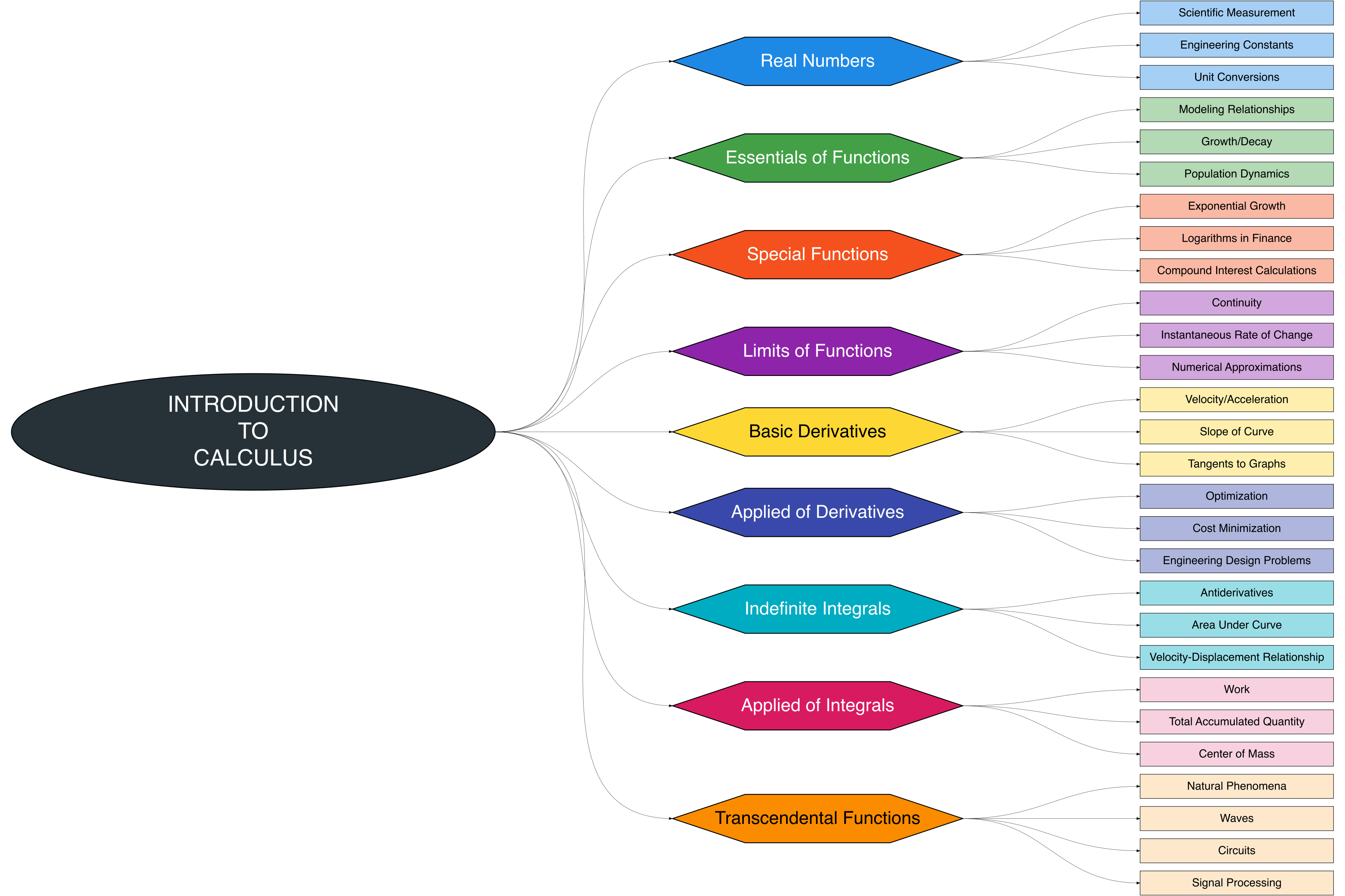
The Figure 1.1 presents a visual overview of the chapter, highlighting the structure of key topics and their interconnections. It provides readers with a clear guide to navigate the material and understand how concepts link to applications.
This chapter introduces the fundamental building blocks of calculus, including real numbers, functions, limits, derivatives, integrals, and transcendental functions. Each concept is connected to practical applications to illustrate how calculus underpins real-world problem-solving.
1.1 Real Numbers
Real numbers are the foundation of all calculus concepts, forming the set of numbers that includes integers, fractions, and decimals. They are essential for performing calculations, defining functions, and understanding limits, derivatives, and integrals. A solid understanding of real numbers allows us to work with continuous quantities, measure physical phenomena, and apply mathematical reasoning in real-world contexts. The key properties, descriptions, and typical applications of real numbers are summarized in Table 1.1.
| Property | Description | Example |
|---|---|---|
| Closure | Operations on real numbers yield real numbers | \(a+b, a-b, a\cdot b, a/b\) (if \(b\neq0\)) |
| Order | Real numbers can be compared and ordered | \(a < b\) → comparing magnitudes |
| Density | There is always another real number \ between two numbers | \(\exists c: a < c < b\) \ → interpolation |
| Absolute Value | Measures distance from zero | \(\lvert a \rvert\) → distance from zero |
| Scientific Measurement | Represent measurable physical quantities | \(g = 9.8\,\text{m/s}^2\) |
| Engineering Constants | Constants used in formulas \ and modeling | \(E\), \(c = 3\times10^8\,\text{m/s}\) |
1.2 Essentials of Functions
Functions describe relationships between variables, showing how one quantity changes with another. They are fundamental in calculus as they provide mathematical models for dynamic systems, patterns, and processes across science, engineering, and economics. A proper understanding of functions requires knowledge of their domain, range, types, and behavior. An overview of the key concepts, descriptions, and applications is given in Table 1.2.
| Key Concept | Description | Example / Application |
|---|---|---|
| Definition | Maps each \(x\) in domain to a unique \(y\) in range | \(f: x \mapsto y\) |
| Domain and Range | Domain = all possible inputs, Range = all outputs | \(x \in [0,10], f(x) \in [0,100]\) |
| Linear Function | Straight-line relationship | \(f(x) = mx + b\) |
| Quadratic Function | Parabolic relationship | \(f(x) = ax^2 + bx + c\) |
| Polynomial Function | Sum of powers of \(x\) | \(f(x) = a_n x^n + \dots + a_0\) |
| Exponential Function | Rapid growth or decay | \(P(t) = P_0 e^{rt}\) \ (population growth) |
| Trigonometric Function | Models periodic behavior | \(T(t) = T_{avg} + A \sin\left(\tfrac{2\pi}{24} t\right)\) \ (temperature changes) |
1.3 Special Functions
Special functions are widely used in science, engineering, and applied mathematics because they model specific natural or engineered phenomena. Extending beyond simple polynomials, they play a central role in solving real-world problems across physics, chemistry, biology, and finance. A structured overview of their main types, descriptions, and applications is provided in Table 1.3.
| KeyConcept | Description | ExampleApplication |
|---|---|---|
| Exponential Functions | \(f(x) = a e^{bx}\); models growth and decay | Compound interest: \(A = P e^{rt}\) |
| Logarithmic Functions | \(f(x) = \log_b(x)\); inverse of exponential | pH scale, sound intensity measurements |
| Trigonometric Functions | \(f(x) = \sin x, \cos x, \tan x\); models periodic behavior | Pendulum motion: \(\theta(t) = \theta_0 \cos(\omega t + \phi)\) |
1.4 Limits of Functions
Limits reveal how functions behave as inputs get closer to a given value. They are essential in calculus, laying the groundwork for derivatives and continuity. With limits, we can explore instantaneous change, refine approximations, and resolve problems where direct evaluation fails. An overview of the main ideas and applications appears in Table 1.4.
| KeyConcept | Description | ExampleApplication |
|---|---|---|
| Definition | \(\lim_{x \to a} f(x) = L\); the value \(f(x)\) approaches as \(x \to a\) | Approximating function values: \(\lim_{x \to 0} \tfrac{\sin x}{x} = 1\) |
| One-sided Limits | Limits approaching from left (\(x \to a^-\)) or right (\(x \to a^+\)) | Instantaneous velocity from left/right time intervals |
| Continuity | \(f\) is continuous at \(x=a\) if \(\lim_{x \to a} f(x) = f(a)\) | Ensuring smooth motion or consistent output in physical systems |
1.5 Basic Derivatives
Derivatives quantify how a function changes with respect to its input, capturing slopes, rates of change, and tangent behavior. They play a central role in calculus by enabling the analysis of motion, growth, optimization, and a wide range of dynamic processes. Key concepts, descriptions, and applications are summarized in Table 1.5.
| KeyConcept | Description | ExampleApplication |
|---|---|---|
| Definition | \(f'(x) = \lim_{\Delta x \to 0} \frac{f(x+\Delta x)-f(x)}{\Delta x}\); rate of change at \(x\) | Instantaneous velocity: \(v(t) = s'(t)\) |
| Interpretation | Slope of tangent line; instantaneous rate of change | Slope of a hill: \(m = h'(x)\) |
| Basic Rules | Power rule, sum rule, constant multiple rule | \(\frac{d}{dx} x^n = n x^{n-1}\), \(\frac{d}{dx}[f+g] = f' + g'\) |
1.6 Applied Derivatives
Applied derivatives illustrate how differentiation is used to solve real-world problems across engineering, economics, physics, and other fields. By examining rates of change, extrema, and concavity, derivatives provide tools for optimizing processes, predicting behavior, and supporting decision-making. Key concepts, descriptions, and applications are summarized in Table 1.6.
| KeyConcept | Description | ExampleApplication |
|---|---|---|
| Optimization | Find maxima or minima by solving \(f'(x)=0\) \ and checking \(f''(x)\) | Maximize profit: \(P'(x)=0\) |
| Rate of Change | Quantifies how one variable changes \ with respect to another | Velocity: \(v(t)=s'(t)\) |
| Critical Points | Points where \(f'(x)=0\) or undefined; \ used to find maxima, minima, or inflection points | Minimizing cost: \(C'(x)=0\); \ analyzing structure stress |
| Motion Analysis | Derivatives of position give \ velocity and acceleration | \(v(t)=s'(t)\), \(a(t)=s''(t)\) |
1.7 Indefinite Integrals
Indefinite integrals, or antiderivatives, undo the process of differentiation, enabling us to recover the original function from its derivative. They represent accumulated quantities such as displacement, total growth, or total charge. The Table 1.7 below summarizes key concepts, descriptions, and example applications:
| KeyConcept | Description | ExampleApplication |
|---|---|---|
| Definition | \(F'(x) = f(x)\); \(\int f(x) dx = F(x) + C\) | Displacement: \(s(t) = \int v(t) dt\); e.g., \(v(t)=3t^2 \implies s(t)=t^3+C\) |
| Power Rule | \(\int x^n dx = \frac{x^{n+1}}{n+1}+C, n\neq -1\) | Integration of \(x^2\) gives \(\frac{x^3}{3}+C\) |
| Constant Multiple | \(\int c f(x) dx = c \int f(x) dx\) | Multiply constant with integral |
| Sum Rule | \(\int [f(x)+g(x)] dx = \int f(x) dx + \int g(x) dx\) | \(\int (x^2+2x) dx = \frac{x^3}{3}+x^2+C\) |
| Total Accumulation | Accumulation of quantity over time | Revenue: \(\int R(t) dt\) |
1.8 Applied Integrals
Transcendental functions are those that cannot be represented as finite polynomials, including exponential, logarithmic, trigonometric, and inverse trigonometric functions. They play a central role in mathematics, physics, engineering, and the applied sciences by modeling complex natural and engineered phenomena. Key types, descriptions, and example applications are summarized in Table 1.8.
| KeyConcept | Description | ExampleApplication |
|---|---|---|
| Definite Integral | Total accumulation of a quantity over interval \([a,b]\): \(\int_a^b f(x) dx\) | Area under curve: \(\int_0^2 x^2 dx = \tfrac{8}{3}\) |
| Area Under a Curve | Calculates area between function and x-axis | Same as above |
| Physical Applications | Integrals for work, mass, charge, revenue | Mass: \(M = \int_a^b \rho(x) dx\), Work: \(W = \int_a^b F(x) dx\) |
1.9 Transcendental Functions
Transcendental functions are functions that cannot be expressed as finite polynomials. They include exponential, logarithmic, trigonometric, and inverse trigonometric functions, and are essential in advanced mathematics, physics, engineering, and applied sciences for modeling complex phenomena. Transcendental functions are used to model complex phenomena in science and engineering in the table Table 1.9.
| KeyConcept | Description | ExampleApplication |
|---|---|---|
| Exponential Functions | \(f(x) = e^x\) or \(a^x\), model growth and decay | RC circuit voltage: \(V(t) = V_0(1 - e^{-t/RC})\) |
| Logarithmic Functions | \(f(x) = \ln x\) or \(\log_a x\), used in scaling | Measuring pH, sound intensity |
| Trigonometric Functions | \(f(x) = \sin x, \cos x, \tan x\), model periodic behavior | Wave motion: \(y(x,t) = A \sin(kx - \omega t)\) |
| Inverse Trigonometric Functions | \(f(x) = \arcsin x, \arccos x, \arctan x\), solving angles | Population oscillations: \(P(t) = P_\text{avg} + A \cos(\omega t + \phi)\) |