Chapter 3 2021.10.06. Exercise
library(ggplot2)a_plot <-
ggplot(mpg, aes(x = model, y = hwy, fill = manufacturer)) +
geom_boxplot() +
theme(axis.text.x = element_text(angle = 30))
a_plot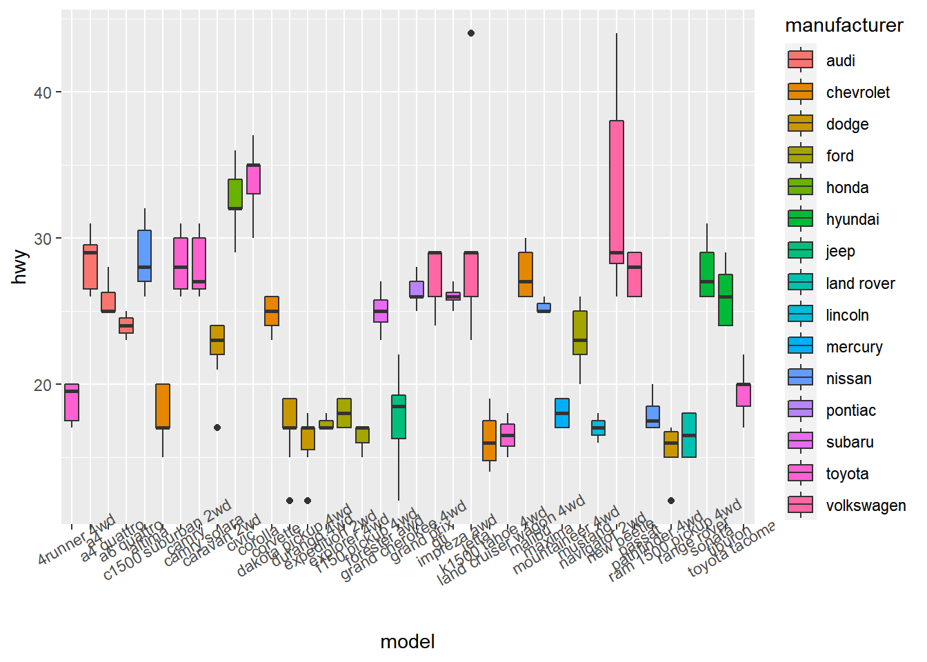
a_plot +
  labs(fill = "Brand")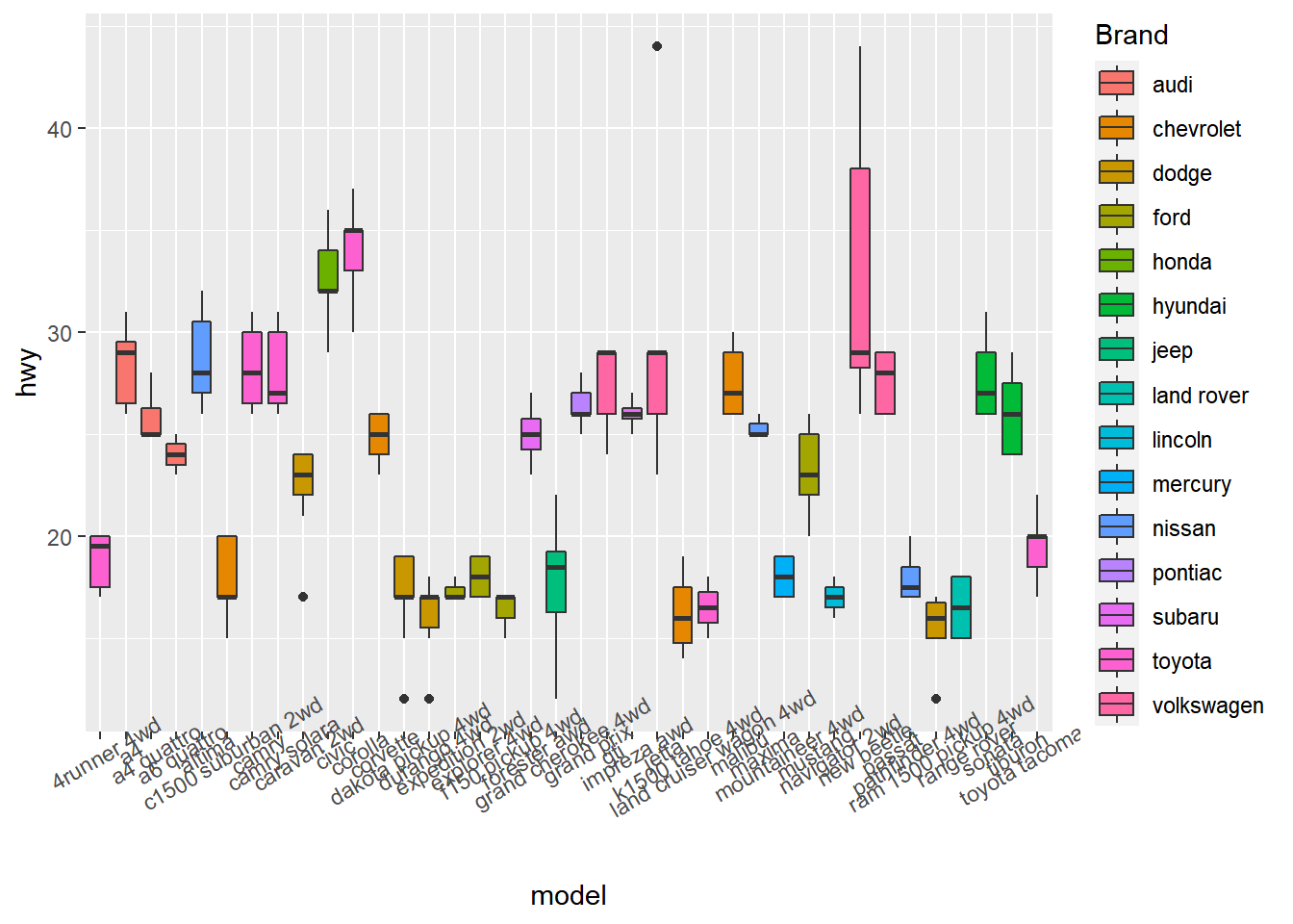
a_plot +
  labs(title = "Counts of Car Class",
       subtitle = "By manufacturer",
       caption = "source: mpg data from ggplot2",
       fill = "Car Company",
       x = "Class of Cars",
       y = "Count")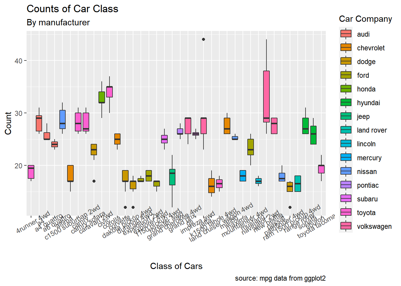
3.1 Exercise 1(with answers)
library(gcookbook)head(heightweight)## sex ageYear ageMonth heightIn weightLb
## 1 f 11.92 143 56.3 85.0
## 2 f 12.92 155 62.3 105.0
## 3 f 12.75 153 63.3 108.0
## 4 f 13.42 161 59.0 92.0
## 5 f 15.92 191 62.5 112.5
## 6 f 14.25 171 62.5 112.0ggplot(heightweight, aes(x = ageYear, y = heightIn, size = weightLb, color = sex)) + geom_point()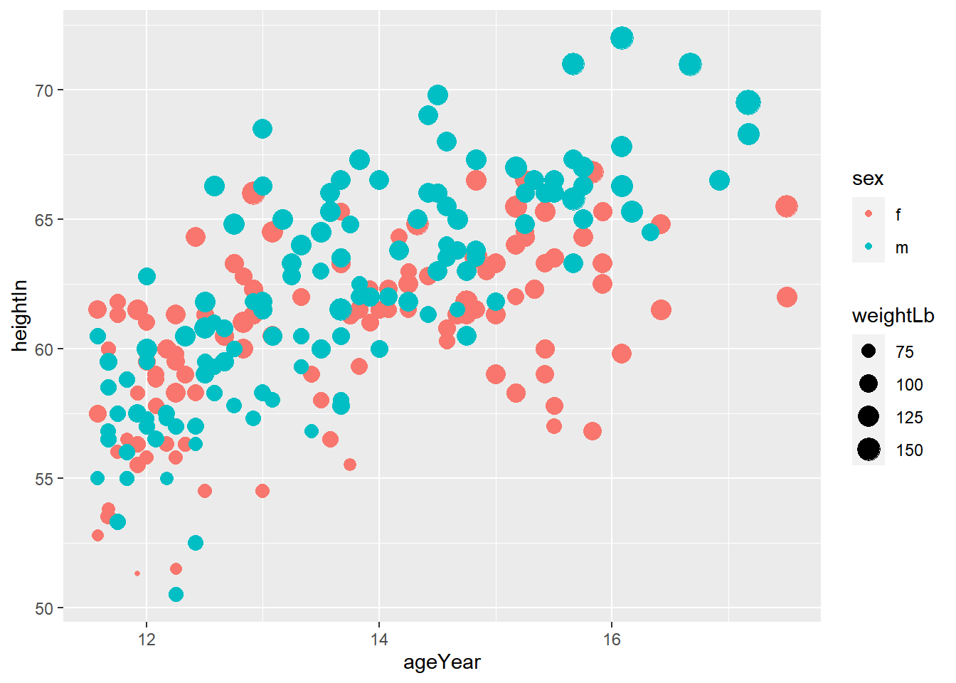
ggplot(heightweight, aes(x = ageYear, y = heightIn, size = weightLb, color = sex)) + geom_point(alpha = 0.3)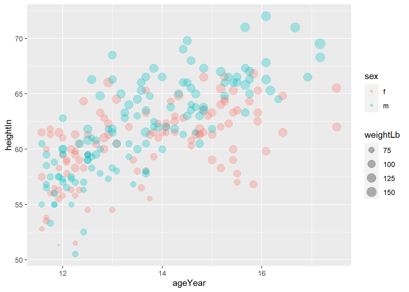
ggplot(heightweight, aes(x = ageYear, y = heightIn, size = weightLb, color = sex)) +
  geom_point(alpha = 0.3) +
  labs(title = "Height and weight of school children",
       subtitle = "Height vs Weight",
       caption = "Source: heightweight",
       x = "Age (year)",
       y = "Height (inchess)",
       size = "Weight (Lb)",
       color = "Gender")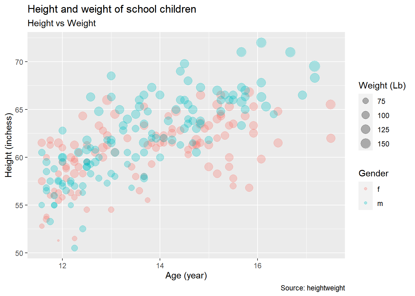
ggplot(heightweight, aes(x = ageYear, y = heightIn, size = weightLb, color = sex)) +
  geom_point(alpha = 0.3) +
  labs(title = "Height and weight of school children",
       subtitle = "Height vs Weight",
       caption = "Source: heightweight",
       x = "Age (year)",
       y = "Height (inchess)",
       size = "Weight (Lb)",
       color = "Gender") +
  theme_classic()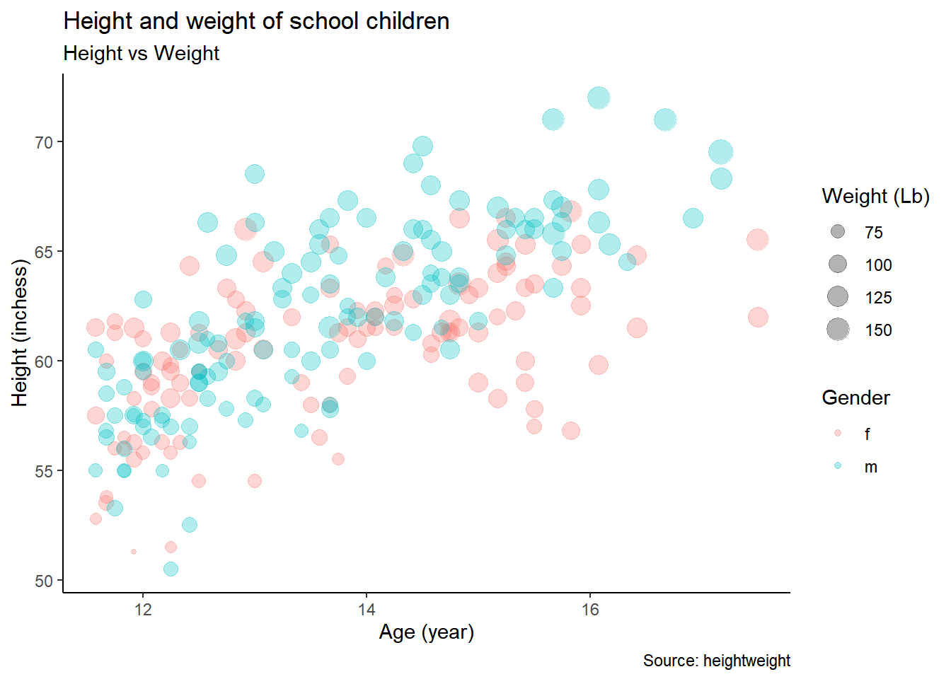
3.2 Exercise 2 (with answers)
ggplot(heightweight, aes(x = heightIn)) +
  geom_histogram()
## `stat_bin()` using `bins = 30`. Pick better value with `binwidth`.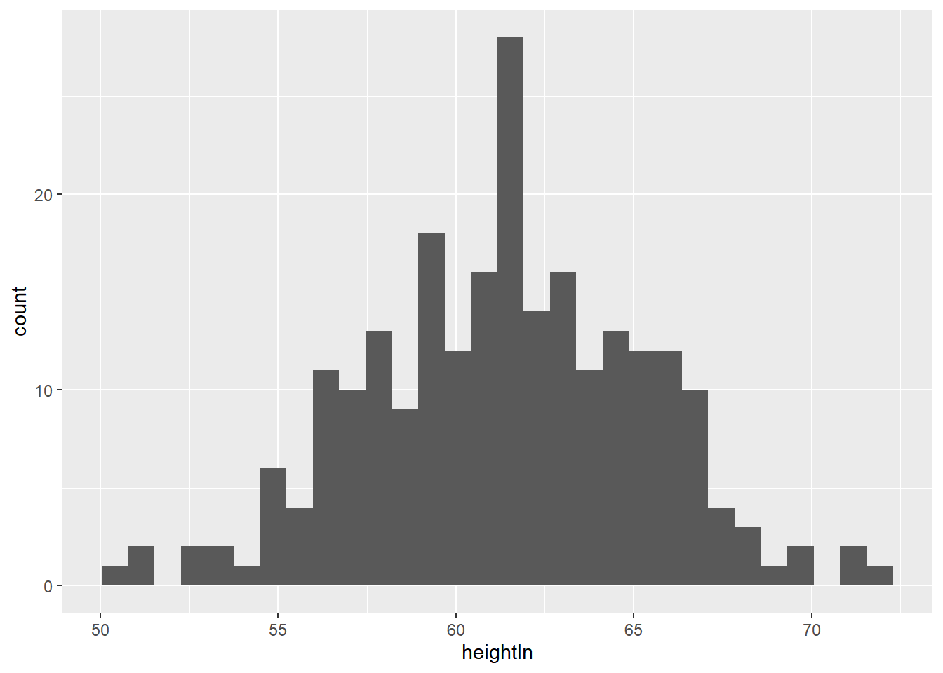
ggplot(heightweight, aes(x = weightLb, fill = sex)) +
  geom_histogram()
## `stat_bin()` using `bins = 30`. Pick better value with `binwidth`.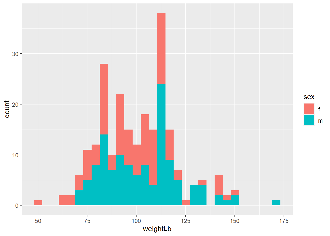
ggplot(heightweight, aes(x = weightLb, fill = sex)) +
  geom_histogram(alpha = 0.4) +
  scale_fill_manual(values = c("orange", "yellow"))
## `stat_bin()` using `bins = 30`. Pick better value with `binwidth`.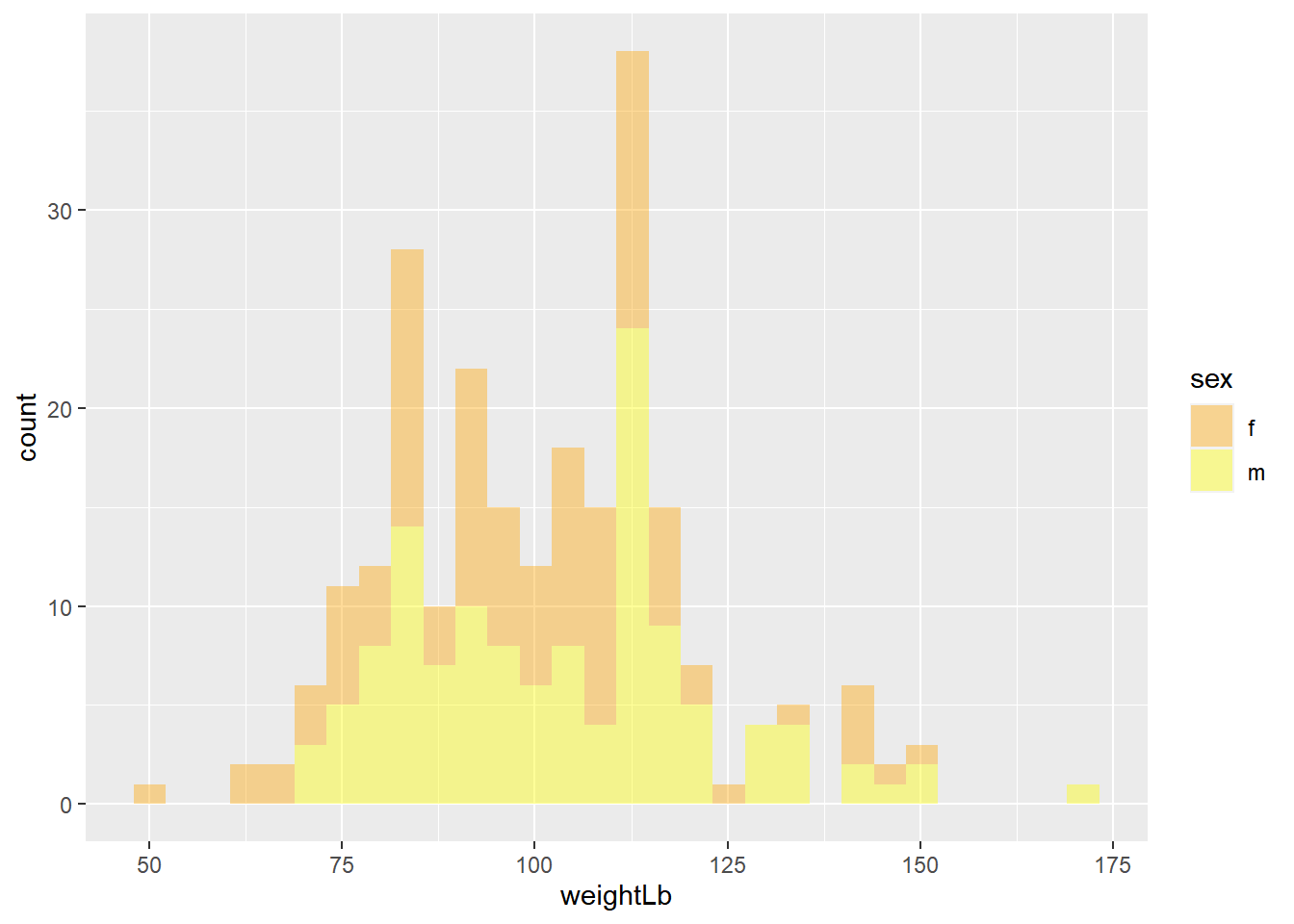
ggplot(heightweight, aes(x = weightLb, fill = sex)) +
  geom_histogram(alpha = 0.4) +
  scale_fill_manual(values = c("orange", "yellow")) +
  labs(title = "A histogram of the weight of school children",
       subtitle = "By gender",
       x = "Weight (Lb)",
       y = "Count",
       fill = "Gender"
  ) +
  theme_minimal()
## `stat_bin()` using `bins = 30`. Pick better value with `binwidth`.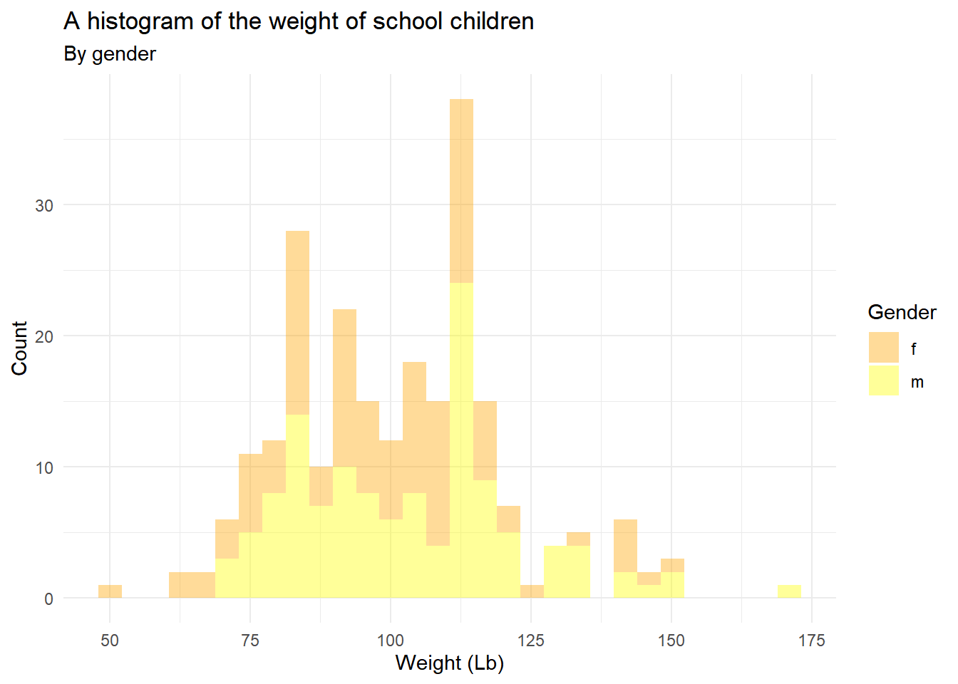
3.3 Exercise 3
head(mpg)## # A tibble: 6 x 11
## manufacturer model displ year cyl trans drv cty hwy fl
## <chr> <chr> <dbl> <int> <int> <chr> <chr> <int> <int> <chr>
## 1 audi a4 1.8 1999 4 auto(~ f 18 29 p
## 2 audi a4 1.8 1999 4 manua~ f 21 29 p
## 3 audi a4 2 2008 4 manua~ f 20 31 p
## 4 audi a4 2 2008 4 auto(~ f 21 30 p
## 5 audi a4 2.8 1999 6 auto(~ f 16 26 p
## 6 audi a4 2.8 1999 6 manua~ f 18 26 p
## # ... with 1 more variable: class <chr>ggplot(mpg, aes(x = hwy, fill = drv)) +
geom_histogram(alpha = 0.5) +
facet_grid(drv~ .) +
labs(title = "Histogram using facet_grid()",
subtitle = "Histogram of Highway Mile Per Gallon"
) +
theme_minimal()## `stat_bin()` using `bins = 30`. Pick better value with `binwidth`.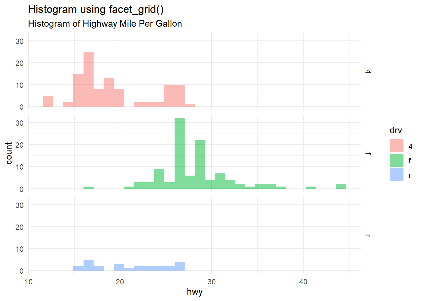
##Exercise 4
library(ggplot2)
options(scipen = 999)
head(midwest)
## # A tibble: 6 x 28
## PID county state area poptotal popdensity popwhite popblack
## <int> <chr> <chr> <dbl> <int> <dbl> <int> <int>
## 1 561 ADAMS IL 0.052 66090 1271. 63917 1702
## 2 562 ALEXANDER IL 0.014 10626 759 7054 3496
## 3 563 BOND IL 0.022 14991 681. 14477 429
## 4 564 BOONE IL 0.017 30806 1812. 29344 127
## 5 565 BROWN IL 0.018 5836 324. 5264 547
## 6 566 BUREAU IL 0.05 35688 714. 35157 50
## # ... with 20 more variables: popamerindian <int>, popasian <int>,
## # popother <int>, percwhite <dbl>, percblack <dbl>,
## # percamerindan <dbl>, percasian <dbl>, percother <dbl>,
## # popadults <int>, perchsd <dbl>, percollege <dbl>,
## # percprof <dbl>, poppovertyknown <int>, percpovertyknown <dbl>,
## # percbelowpoverty <dbl>, percchildbelowpovert <dbl>,
## # percadultpoverty <dbl>, percelderlypoverty <dbl>, ...options(scipen = 999)
ggplot(midwest, aes(x = area, y = poptotal)) +
geom_point(aes(size = popdensity, color = state), alpha = 0.4) +
geom_smooth(method = "auto", se=F) +
xlim(c(0, 0.1)) +
ylim(c(0, 500000)) +
labs(title = "Scatterplot",
subtitle = "Area vs Population",
caption = "Source: midwest",
x = "Area",
y = "Population") +
theme_classic()## `geom_smooth()` using method = 'loess' and formula 'y ~ x'## Warning: Removed 15 rows containing non-finite values (stat_smooth).## Warning: Removed 15 rows containing missing values (geom_point).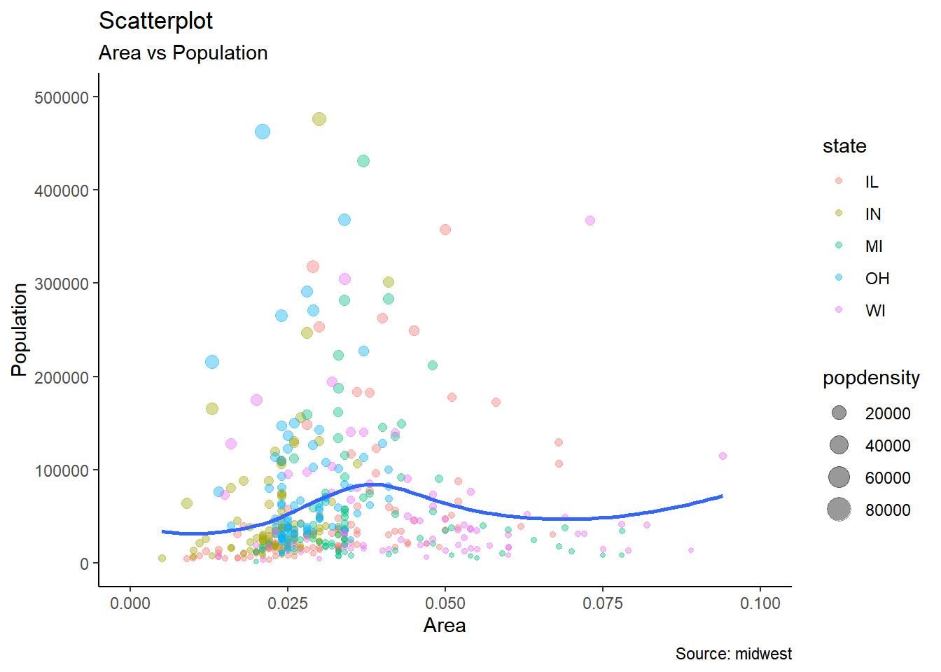
3.4 Exercise 5
library(datasets)
str(iris)
## 'data.frame': 150 obs. of 5 variables:
## $ Sepal.Length: num 5.1 4.9 4.7 4.6 5 5.4 4.6 5 4.4 4.9 ...
## $ Sepal.Width : num 3.5 3 3.2 3.1 3.6 3.9 3.4 3.4 2.9 3.1 ...
## $ Petal.Length: num 1.4 1.4 1.3 1.5 1.4 1.7 1.4 1.5 1.4 1.5 ...
## $ Petal.Width : num 0.2 0.2 0.2 0.2 0.2 0.4 0.3 0.2 0.2 0.1 ...
## $ Species : Factor w/ 3 levels "setosa","versicolor",..: 1 1 1 1 1 1 1 1 1 1 ...ggplot(iris, aes(x=Sepal.Length, y=Sepal.Width))+
geom_point(aes(color=Species, shape=Species), alpha = 0.5, size = 6) +
labs(title = "Scatterplot",
subtitle = "Sepal.Length Vs Sepal.Width",
caption = "Source: iris") +
theme_minimal()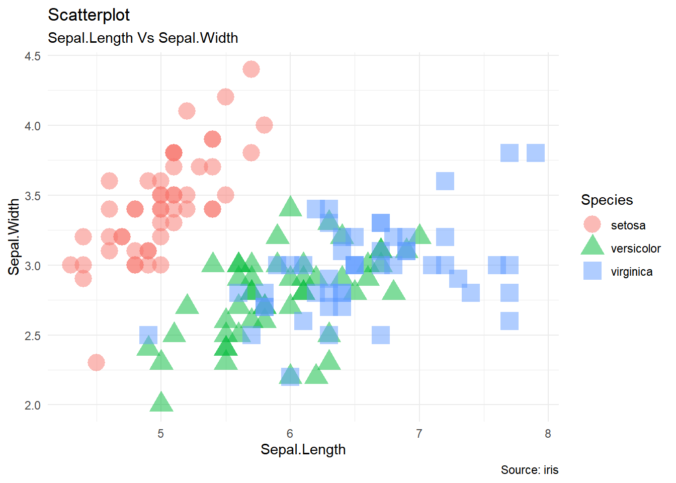
3.5 Exercise 6
library(gcookbook)ggplot(heightweight, aes(x = heightIn, y = weightLb, color = sex)) +
geom_point(size = 3, alpha = 0.5) +
geom_smooth(method = lm, se=F) +
labs(title = "Scatterplot",
subtitle = "Height vs Weight",
caption = "Source: heightweight") +
theme_classic()## `geom_smooth()` using formula 'y ~ x'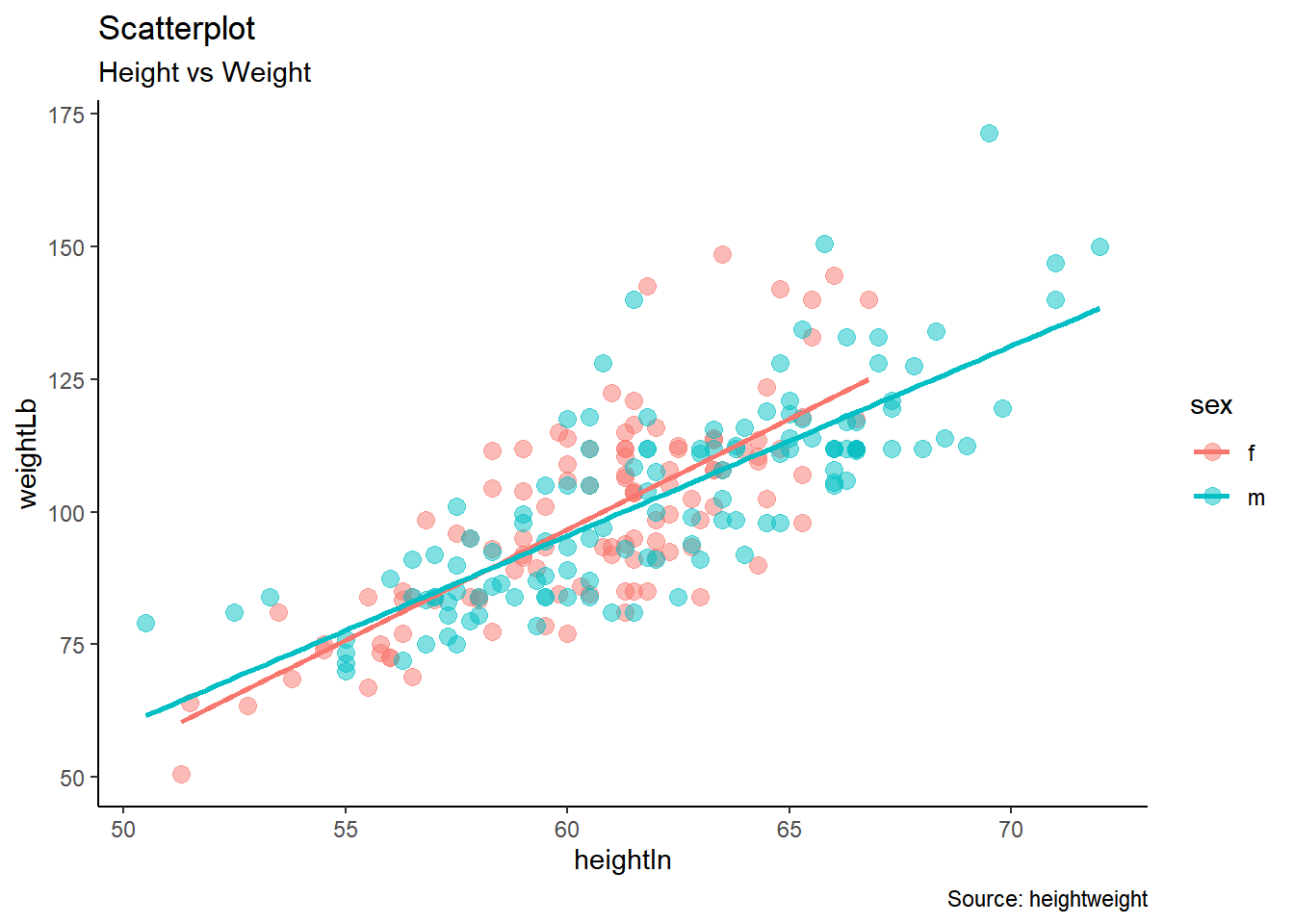
3.6 Exercise 7
library(RColorBrewer)
ggplot(mpg, aes(x=manufacturer)) +
  geom_bar(aes(fill=class), width = 0.5) +
  theme_minimal() +
  theme(axis.text.x = element_text(angle = 65)) +
  labs(title = "Barplot",
       subtitle = "Manufacturer across vehicle Classes") +
  scale_fill_brewer(palette = "Spectral")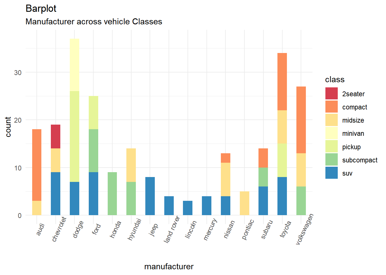
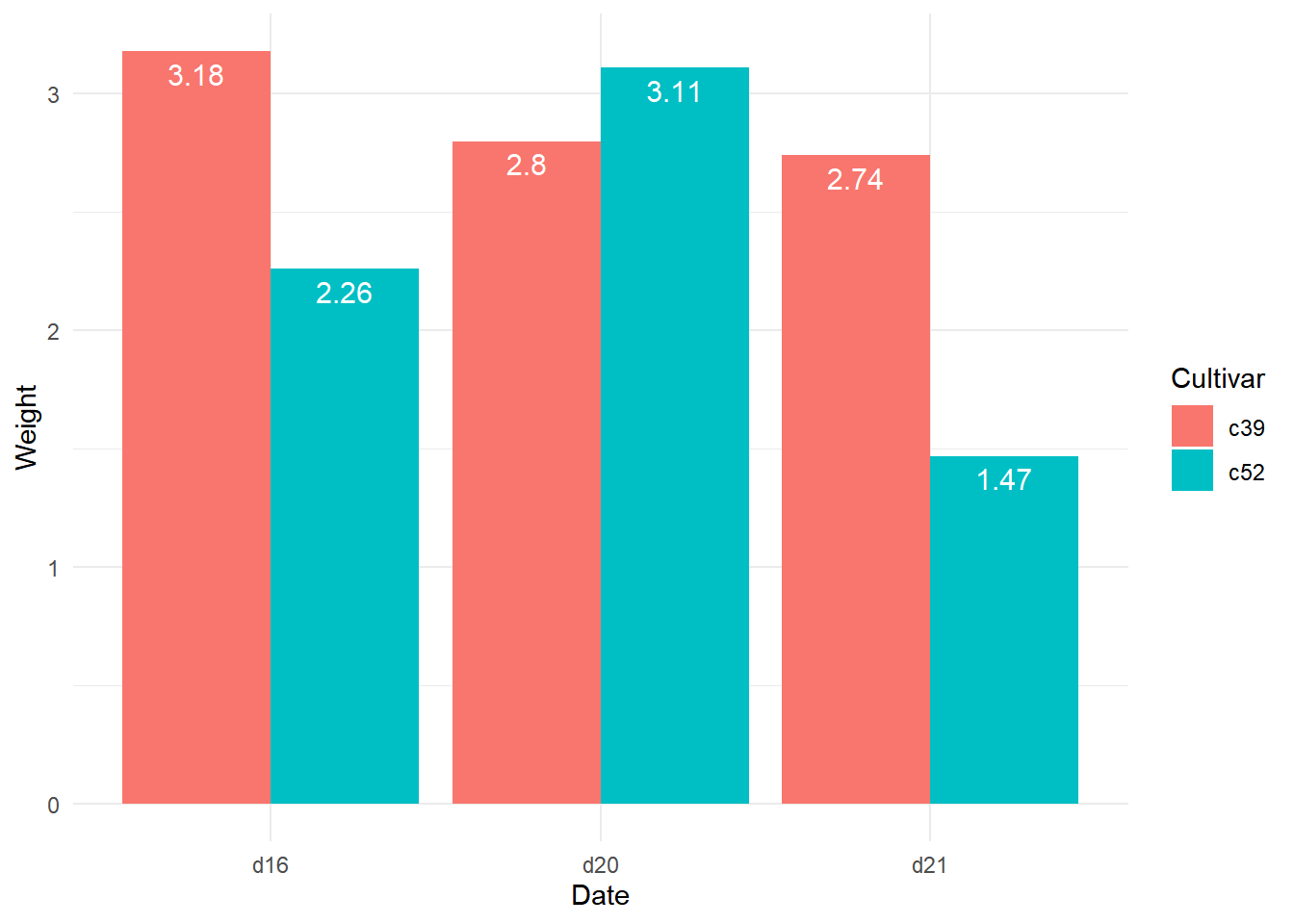
3.7 Exercise 8
ggplot(cabbage_exp, aes(x = Date, y = Weight, fill = Cultivar)) +
  geom_col(position = "dodge") +
  geom_text(aes(label = Weight), colour = "white", size = 4, vjust = 1.5, position = position_dodge(.9)) +
  theme_minimal()