2.1 Basic structures
2.1.1 Maths
Maths is written exactly as expected from LateX by using dollars signs, e.g. \(\sum_{i=1}^n i = \frac{n(n+1)}{2}\). You can use display maths as usual, e.g. let \(p\in \mathbb{Z}_{>0}\) then \[\lim_{n\to\infty}\left(\sum_{i=1}^n \frac{1}{i^p}\right) = \begin{cases} \infty & p=1 \\ \zeta(p) & p>1\end{cases}.\] You can number equations by using the usual backslash ‘begin{equation}’ command - however they must have a label with the prefix ‘eq:’, see (2.1):
\[\begin{equation} f\left(k\right) = \binom{n}{k} p^k\left(1-p\right)^{n-k} \tag{2.1} \end{equation}\]
Bookdown also understand the ‘\begin{align}’ command:
\[\begin{align*} x\in (A^c)^c &\iff \neg(x\in A^c)\\ &\iff \neg(x\not\in A)\\ &\iff x\in A. \end{align*}\]
The key bit is that there should be no empty space between the dollar signs and the first and last maths symbols (otherwise ‘knitr’ does not recognise you are typing maths).
Unfortunately, there is no easy way to implement macros for the moment (that can be compiled in both PDF and HTLM), so you will need to write full latex commands - e.g., ‘\mathbb{R}’ as opposed to ‘\R’.
2.1.2 Lists
- Example of a numbered list
- With a bullet point list nested in
- second item in the bullet point list
- second item in the numbered list
- with a nested numbered list
- Note that an empty line is needed before the start and end of the list.
2.1.3 Tables
| Heading 1 | Heading 2 | Heading 3 |
|---|---|---|
| left aligned column | centered aligned | right aligned |
| \(\frac{1}{2}\) | \(x^2+2\) | non-maths entry |
Note that the row :--|:--:|--:| as well being used to define how columns are aligned (by the usage of :) is also used to
define the relative (not absolute) size of each column (by the usage of -).
2.1.4 Pictures
You can include pictures stored on your computer, see Figure 2.1.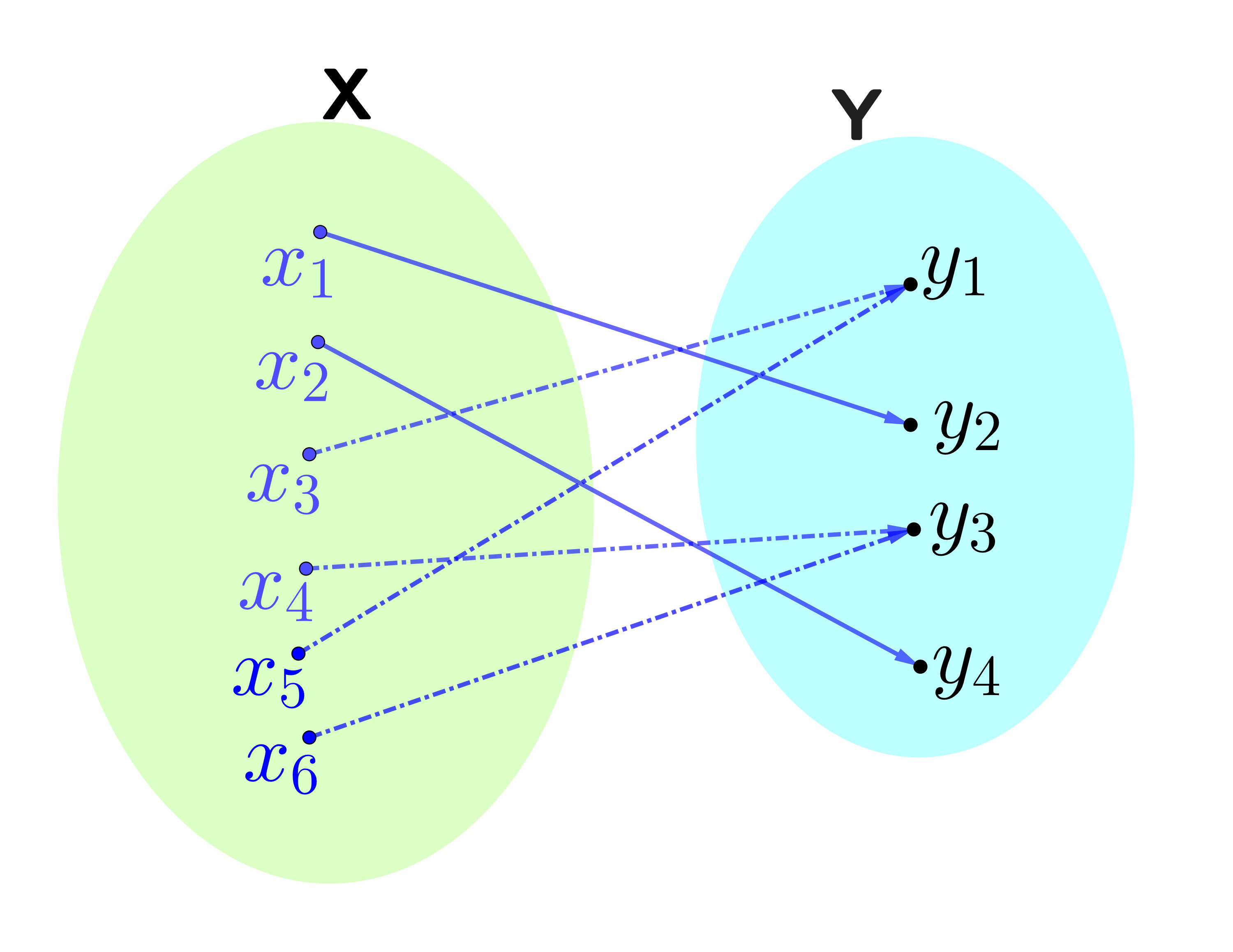
Figure 2.1: A surjective but not injective function \(\mathfrak{f}\) - made using Geogebra
Note the use of a double backslash when using maths inside the caption (as an escape character).
Note that it is good practice to always include an alternative text describing the picture.
RStudio can also understand tikzpicture code. However this needs the package pdftools. So the example below is commented out, but you can un-comment it once you’ve run the following line in RStudio Console:
install.packages(“pdftools”)
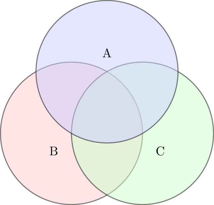
Figure 2.2: A Venn Diagram - made using Tikz
Note: What happens is that RStudio creates the picture and saves it, then adds a ‘include graphic’ command pointing to the picture. However, due to file path issues, once you’ve compile any new pictures I recommend you copy across the folder ‘Figures’ and ‘[Lecture Note title]-files’ into the ‘Lecture Notes’ folder.