4 Script

4.1 CPS

I elected to separate our data analysis process into two overarching sections: (1) the main analysis, and (2) the breakdowns. The main analysis describes the portion of this project that is a direct continuation of the work published by Louise and Nasiha in 2022. It simply examines disability incidence, labor force participation, and telework rates for people with disabilities for the overall population and by age group.

The breakdowns component conducts further analysis by population sub-group – gender, education, geography, etc. It also includes analysis related to ongoing and new disabilities, specific age dynamics, and transitions into and out of the labor force.

This chapter is meant to describe the purpose of each do-file used to execute the “main analysis” and the “breakdowns.”

4.1.1 Main Analysis

The “main analysis” section of this project is based heavily on a paper authored by Louise and Nasiha in 2022. They use data from the Current Population Survey (CPS) to assess the effects of long COVID and remote work on the labor force participation and work hours of people with disabilities. The code uses data from the CPS to calculate age-adjusted disability incidence and participation rates, telework, and average weekly hours for those with disabilities, as well as several other labor force statistics (employment, unemployment, etc.). This research focuses primarily on telework, participation, and disability incidence.

There are three do-files associated with the “main analysis”:

data_clean.do: The objective of this script is to read in our raw data, clean it, and produce several key statistics at a monthly rate from May 2008 until the most recent CPS data release. To account for the effects of population aging, we age-adjust each of our outputs. By “reweighting” the data to a standard age distribution, we ensure that changes in disability over time do not result only from population aging. It creates a final data set called cleaned_bynewtime.dta, which contains all of our statistics at a monthly rate for the overall population and for several age sub-groups. Our statistics of interest are the following:

Age-adjusted disability rates (overall disability and by disability type)
Age-adjusted labor force participation for those with disabilities (for overall disability and for each specific type of disability)
Age-adjusted telework rates for those with disabilities (for overall disability and for each specific type of disability)

In addition to these primary results, this code also generates other statistics such as average hours, employment, unemployment, etc.

analysis.do: In this do-file, we use the final .dta file created by data_clean.do to augment our analysis. cleaned_bynewtime.dta simply contains the age-adjusted rates of disability, telework, participation, etc. In this script, we execute tasks like calculating the percentage point change in the disability rate since 2019. For the most part, the sections of this code are self-explanatory.

tables_figures.do: This do-file exports the data created in analysis.do to Excel. This is our preferred way to examine the results – this way you can easily show Louise the underlying data. This code exports the data used in the tables/figures that appear in 2022 paper – some of these we no longer care about. As you read through the script, you’ll notice I’ve commented out large sections that we don’t typically look at. Here are the figures we actually care about:

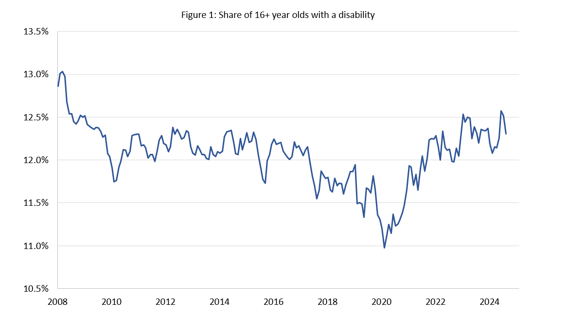
Figure 1 (overall disability rate)
Figure 2 (overall disability rate by age)
Figure 3 (labor force participation rates by age for the overall disability population)
Figure 7 (disability rates by age and disability type)
Figure 8 (participation rates by age and disability type)
Figure 9 (telework rate)

The code exports the results to an Excel sheet that I’ve pre-formatted, so the new data should automatically populate the graphs without you having to format anything.

The main analysis code makes charts that look like this:

4.1.2 Breakdowns

4.1.2.1 individual_disabilities.do

This do-file is an extension of the main analysis, but it redefines our disability categorizations to include only people that have one disability (i.e. they only have a hearing disability, or only have a cognition disability, etc.). The code is practically identical to the do-files mentioned in section 4.1.1. Instead of rewriting the age distribution data we use to age-adjust our results, it simply calls the age distribution data defined by the data_clean.do (data_raw/ageshares.dta). So make sure you’ve run that script first!

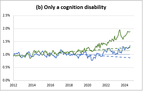
individual_disabilities.do first defines disability indicator variables for those that have ONLY one particular disability and then calculates age-sex-adjusted disability incidence and participation. All intermediate datasets are included in the breakdowns\one_disability sub-folder. As I said above, we do not recalculate the age shares for this analysis! The resulting data is outputted to our main results Excel file. They are titled “Figure 7a.1” and “Figure 7a.2” in Long COVID\CPS\output\spreadsheets\tables_figures.xlsx.

Here is an example of a graph produced by this do-file:

4.1.2.2 dot_plots.do

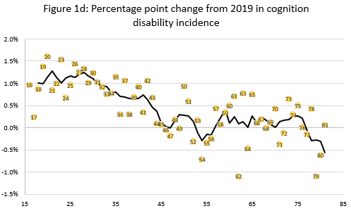
This script calculates the percent and percentage point change from 2019 in disability incidence and labor force participation. It reads in our raw data, calculates average rates of disability/participation by year and age, and then calculates the changes from 2019 for each age. All intermediate datasets are stored in breakdowns\age and the results are outputted to dot_plots.xlsx in the age sub-folder.

Here is an example of a graph produced by this script:

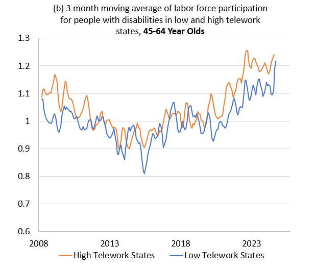
4.1.2.3 tel_state.do

This script calculates age-adjusted disability incidence and labor force participation for two groups of states: (1) states with “high” telework rates and (2) states with low telework rates. We want to see if LFPR has changed more/less depending on the telework prevalence in a state. A high telework state is a state that’s telework rate is above median (in the distribution of state telework rates in 2023). A low telework state has a rate below median. We define two age distributions for our age adjustment procedure - an age distribution for the subpopulation that lives in high telework states and an age distribution for the subpopulation that lives in low telework states. When we calculate our sub-group-specific participation and disability rates, we age adjust based on the population shares of these two respective sub-groups in 2019. The script concludes by outputting the cleaned data to an excel file called tel_state_tables_figures.xlsx.

Note: The code simply outputs raw rates. You’ll notice in the Long COVID slides we do things like normalizing the data and calculating the three month moving average in Excel. Not the cleanest, I know, but a lot of these adjustments occurred as Louise and I were reviewing the data in Excel and making ad hoc changes. Feel free to code it.

Here is an example of a graph produced by this script:

4.1.2.4 ongoing.do

In this do-file, we exploit the panel structure of the CPS to track the disability and labor force status of the same individuals over time. Recall that in the CPS, respondents are surveyed for four months, excluded for the next eight, and then surveyed again for another four months. For individuals in their second survey round, we can observe their disability status from 12 months prior.

In this do-file we calculate disability incidence and labor force participation for individuals with four statuses:

New Disability - They are disabled now but did not have a disability 12 months ago.
Ongoing Disability - They are disabled now and also had a disbaility 12 months ago.
Un-Disabled - They do not have a disability now but had one 12 months ago.
Never disabled - They do not have a disability now and did not have one 12 months ago.

In the IPUMs data, individuals are identified with a person-level code: cpsidp. We use a self-merge to match our data on the individual level to the observation for that same person 12 months prior. mish is an IPUMs-defined variable for “month in survey” that allows us to easily match individuals to themselves 12 months ago. Keep in mind that many respondents do not respond to all months of the survey, resulting in missing observations. We omit those who cannot be matched.

The code calculates disability and labor force participation for the four groups above. The rates are age-adjusted (age-adjust only, not sex). Intermediate data is stored in the breakdowns\ongoing subfolder. The results are outputted in ongoing_figures.xlsx in the ongoing subfolder.

Here is an example of a graph produced by this script:

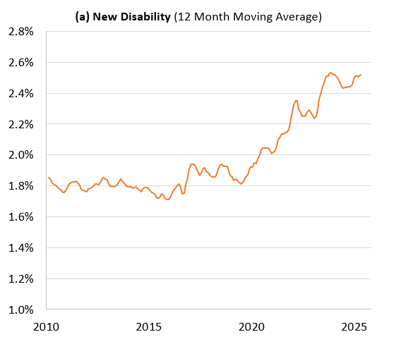
Note: I calculated the 12-month moving average in Excel, but feel free to code that if you want to.

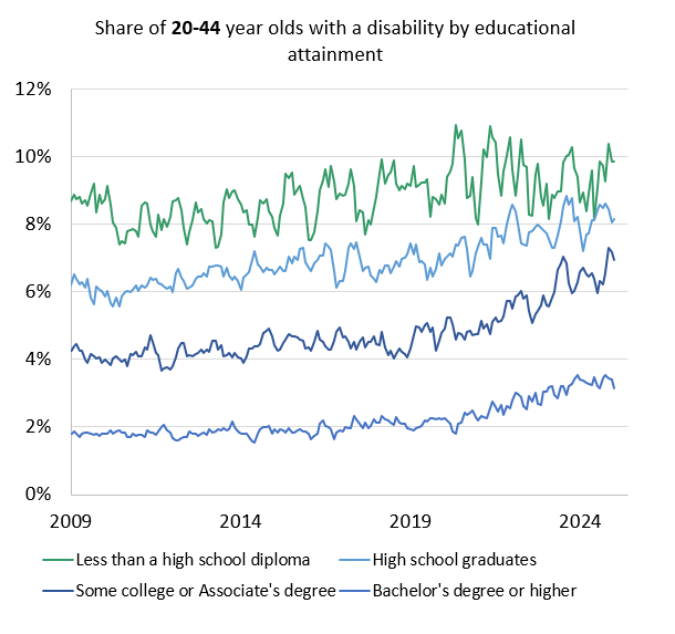
4.1.2.5 education.do

The objective of this do-file is to execute our analysis of disability incidence and participation by education status. The code divides the population into 4 groups based on a respondent’s highest level of educational attainment: (1) Less than a high school diploma, (2) High school diploma or equivalent, (3) Some college or Associate’s Degree, and (4) Bachelor’s degree or higher. We calculate labor force participation and disability incidence for each of these groups.

The do-file proceeds in three sections (very similar to the main analysis). The first section, called “Data Clean”, pulls in the raw CPS data and prepares it for analysis. It outputs a dataset called cleaned_bynewtime to the education sub-folder, which contains the monthly disability and labor force participation rates by age group and education status. The second section is called “Analysis”, which further prepares the monthly levels by age and education. The final section is called “tables_figures”, which exports the monthly levels to an Excel sheet in the breakdowns\education sub-folder. All intermediate files are stored in breakdowns\education\data. All final datasets are stored in breakdowns\education\output\datasets. The resulting Excel file, called education_figures.xlsx is stored in breakdowns\education\output\spreadsheets.

The results are age adjusted using 2019 population shares. For this breakdown, however, we age adjust separately within each of the four education groups defined above. For example, we age-adjust the labor force participation rate (LFPR) for individuals with a high school diploma using the 2019 age distribution of the population with a high school diploma. This allows us to remove the effects of age trends within each education sub-group.

Here is an example of a graph produced by this code:

4.1.2.6 occupation_crosswalk.do and occupation_shares.do

We use occupation_crosswalk.do and occupation_shares.do to examine changes in the share of the population employed in what we define as “teleworkable” jobs. The CPS includes hundreds of detailed occupation codes, and we classify each occupation as either “remote workable” or “not remote workable.” Using these classifications, we calculate the share of people with disabilities employed in remote workable jobs over time. The employment shares are age adjusted. The goal is to assess the role of remote work in helping people with disabilities enter or remain in the labor force. Unlike the actual remote work variable (included in the CPS only after the pandemic), we have pre-pandemic data for job type. Whether a person’s job is remote workable serves as a proxy for whether they worked remotely.

occupation_crosswalk.do

occupation_crosswalk.do is the first script you must run in order to execute this analysis. It uses data from the Occupational Information Network (O*NET), a free online database that contains information on hundreds of jobs (the skills and knowledge required for the job, the typical work activities, etc.). We use methodology and code written by Dingel and Neiman (2022) to develop a measure of a job’s remote workability based on information from the O*NET database of worker and occupation attributes. The code uses the “Occupation Data”, “Work Context”, and “Work Activities” datasets published by O*NET. You can access the data here. This code is equipped to handle data version 24.2. The code expects raw .txt files.

You can access the Dingel and Neiman (2022) Github reposity here if you are interested in reading more about their code.

Most of this do-file is copied directly from Dingel and Neiman’s repository linked above. There are comments in the do-file explaining what each section does.

Crosswalking Our Data

O*NET classifies occupations using O*NET-SOC codes, a more granular version of the SOC taxonomy used by OMB and BLS (i.e. O*NET and BLS/OMB use a different system to label occupations.). The BLS SOC taxonomy was updated in 2018, and O*NET updated its O*NET-SOC classification to reflect these changes. This code uses the 2010 O*NET-SOC and 2010 SOC codes rather than the updated version (our CPS data we pull from IPUMs uses the harmonized 2010 version of the SOC code (called OCC) because these codes often change over time).

Section 1 of the code classifies jobs as teleworkable, and these occupations are identified by their 2010 O*NET-SOC code.
Section 2 of the code merges the occupations classified by the O*NET-SOC codes with their BLS SOC codes.
Section 3 of the code merges the occupations classified by their SOC codes with the corresponding 2010 OCC codes. OCC is the classificiation system used by the ACS and CPS IPUMS data.

As indicated above, this is a two step crosswalk taking us from the most granular data to the least– we lose some jobs and combine some jobs along the way.

There are some intermediate datasets you’ll need to download to execute all of this crosswalking:

2010_to_SOC_Crosswalk.xlsx: https://github.com/jdingel/DingelNeiman-workathome/blob/master/downloaddata/output/2010_to_SOC_Crosswalk.xlsx
oes_2019_hybrid_structure.xlsx: https://www.bls.gov/oes/oes_2019_hybrid_structure.xlsx
cenocc2010.xlsx: https://www.bls.gov/cps/cenocc2010.htm

It’s not perfect, and you’ll notice at the end of the do-file that I needed to classify some of the occupations manually. The output of this script is a file called occ_teleworkable.dta containing a list of occupations and an indicator variable for whether that job is remote workable. We merge occ_teleworkable.dta with our CPS microdata to calculate employment in remote workable jobs. We lose ~4% of responses doing this merge (because I didn’t finish manually categorizing the unclassified occupations - I figured it was close enough. Sorry, that’s not very responsible of me.)

occupation_shares.do

This script uses the data set created by occupation_crosswalk.do to calculate the employment-to-population ratio and employment shares in remote workable and non-remote workable occupations. We merge our CPS micro data with a binary variable indicating whether individuals have a remote workable job.

This code proceeds in two main sections:

“Data Clean” calculates age-adjusted employmet-to-population ratios for each disability type by job type (remote workable vs. not remote workable). It also gets the age-adjusted share of the employed population that works in a remote workable occupation by age group and disability type.
“Tables & Figures” exports the resulting data to Excel.

All intermediate files are stored in breakdowns/occupation/

The resulting Excel file is breakdowns/occupation/output/spreadsheets/occ_tables_figures.xlsx

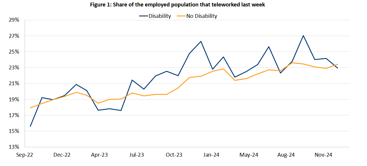
Here is an example of a graph created by this do-file:

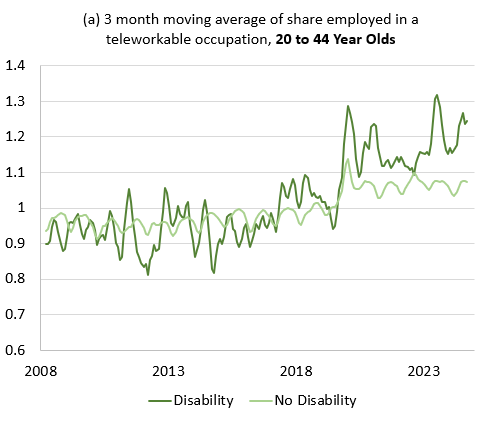
Note: I calculated the 3-month moving average in Excel – feel free to code that up if you want to

4.1.2.7 absences.do

In this do-file, we calculate the share of the population that reports being out of the labor force due to a disability and the share of the employed population that was absent from work last week due to illness. These rates are age adjusted using 2019 age shares. The code has three sections: (1) “Data Clean”, which defines key variables, gets our counterfactuals, and calculates the age-adjusted rates, (2) analysis, which prepares the data to be exported, and (3) “Tables & Figures”, which exports the data to Excel.

I created two definitions for “out of the labor force due to a disability.” These definitions are based on two IPUMS variables. The first is EMPSTAT– the generic labor force categorization variable. Respondents that are out of the labor force pick from six categories to explain why: (1) unable to work, (2) housework, (3) school, (4) unpaid, (5) retired, and (6) other. The second variable, NILFACT, labels more specifically why someone is out of the labor force: (1) Disabled, (2) ill, (3) in school, (4) taking care of house or family, (5) Something else. The universe for NILFACT is those that respond “other” to EMPSTAT, so a limited number of respondents are actually asked the question. Based on some IPUMS blog posts, I defined two versions of “not in the labor force due to a disability” (the first one seems more common to use??):

“Unable to Work” (EMPSTAT), “Ill” (NILFACT), “Disabled” (NILFACT)
“Other” (EMPSTAT), “Disabled” (NIFLACT)

All intermediate data sets and outputs are stored in the breakdowns/labor sub-folder. The results are exported to breakdowns/labor/output/spreadsheets/labor_figures.xlsx

Here is an example of a graph generated by this script: Note: I calculated the 12 month moving average in Excel– feel free to code that if you want.

4.1.2.8 transition_tables.do

transition_tables.do calculates age-adjusted flows into and out of the labor force for the disability population. It begins by defining statuses for each possible combination of disability, job, type, and labor force status. We calculate the average value of the share of the population flowing into and out of these statuses from 2017-2019 and 2022-2023 to determine how the rates have changed pre-post pandemic.

We exploit the panel structure of the CPS to track the disability and labor force status of the same individuals over time. Recall that in the CPS, respondents are surveyed for four months, excluded for the next eight, and then surveyed again for another four months. For individuals in their second survey round, we can observe their disability status from 12 months prior. In the IPUMs data, individuals are identified with a person-level code: cpsidp. We use a self-merge to match our data on the individual level to the observation for that same person 12 months prior. mish is an IPUMs-defined variable for “month in survey” that allows us to easily match individuals to themselves 12 months ago. Keep in mind that many respondents do not respond to all months of the survey, resulting in missing observations. We omit those who cannot be matched.

We begin by defining starting states for each combination of disabled/non-disabled and in the labor force/not in the labor force.

Disabled and not in the labor force
Not disabled and not in the labor force
Disabled and in the labor force
Not disabled and in the labor force
Cognitive disability and not in the labor force
Cognitive disability and in the labor force
Physical Disability and not in the labor force - NOTE: in this script, “physical disability” means any non-cognition disability
Physical Disability and in the labor force

We also define starting statuses fo reach combination of disabled/non-disabled and remote workable/non-remote workable occupation. Keep in mind that you must be in the labor force to have an occupation.

Disabled, in the labor force, and not in a remote occupation.
Disabled, in the labor force, and in a remote occupation.
Not disabled, in the labor force, and not in a remote occupation.
Not disabled, in the labor force, and in a remote occupation.
Cognitive disability, in the labor force, and not in a remote occupation
Cognitive disability, in the labor force, and in a remote occupation
Physical disability, in the labor force, and not in a remote occupation
Physical disability, in the labor force, and in a remote occupation

We merge these lagged statuses to the status of the same person 12 months ahead to calculate flows into and out of the labor force. We age-sex adjust these statistics. We calculate these flows for 20-44 year-old and 45-64 year olds. In the tables figures section, we export the data to Excel. Each starting state gets its own sheet, and each disability type gets its own file. Intermediate datasets are stored in breakdowns/transition_tables/.

The Excel outputs are the following:

breakdowns/transition_tables/transition_tables_disy (overall disability result)
breakdowns/transition_tables/transition_tables_remy (cognition disability result)
breakdowns/transition_tables/transition_tables_nremy (physical disability result)

The resulting tables look like this:

4.1.2.9 new_disability_conceptions.do

This do-file executes the same exact calculations as the “main analysis” but with new disability definitions. It defines only four types of disabilities (respondents that ONLY have these types of disabilities):

Hearing
Vision
Physical
Other

I recommend reviewing the main analysis script and documentation if you are not comfortable with what each section of this code accomplishes.

The resulting data (age adjusted participation and disability) is exported to breakdowns/new_disability_conceptions/output/spreadsheets/new_d_tables_figures.xlsx

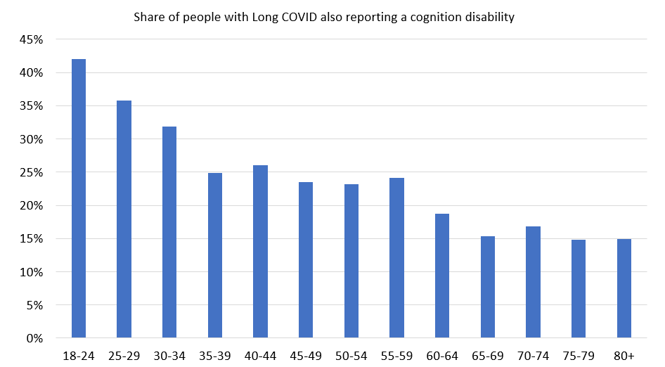
The last section of code generates four tables that summarize the number of individuals with different types of disabilities—vision (eyey), hearing (heary), physical (physy), and other (othery)—by year from 2015 to 2024. The analysis is split into two age groups: adults aged 20–44 and adults aged 45–64. For each group, it first produces raw counts of individuals reporting each disability combination (Tables 1a and 2a), then creates population-weighted counts using survey weights (wtfinl) to reflect national estimates (Tables 1b and 2b). Each set of results is exported to a different sheet in an Excel file. Temporary files are used to store and merge annual data, and then deleted at the end of each block.

They are stored in breakdowns/new_disability_conceptions/output/spreadsheets/disability_counts.xlsx.

4.1.2.10 red_blue_states.do

The objective of this do-file is to execute our analysis of disability incidence and participation for two groups of states: red states and blue states (based on 2020 Biden vote shares).

The do-file has three sections (very similar to the main analysis). The first section, called “Data Clean”, pulls in the raw CPS data and prepares it for analysis. It outputs a dataset called cleaned_bynewtime to the red_blue sub-folder, which contains the monthly disability and labor force participation rates by age group and state. The second section is called “Analysis”, which further prepares the monthly levels by age and state. The final section is called “tables_figures”, which exports the monthly levels to an Excel sheet in the breakdowns\red_blue sub-folder. All intermediate files are stored in breakdowns\red_blue\data. All final datasets are stored in breakdowns\red_blue\output\datasets. The resulting Excel file, called rb_tables_figures.xlsx is stored in breakdowns\red_blue\output\spreadsheets.

The results are age adjusted using 2019 population shares. For this breakdown, however, we age adjust separately within the subgrouping of states defined above. For example, we age-adjust the labor force participation rate (LFPR) for individuals in red states using the 2019 age distribution of the population in red states. This allows us to remove the effects of age trends within each state sub-group.

4.1.2.11 foreign_born.do

The objective of this do-file is to execute our analysis of disability incidence and participation for foreign born workers and native born workers.

The final section is called “tables_figures”, which exports the monthly levels to an Excel sheet in the breakdowns\foreign_born sub-folder. All intermediate files are stored in breakdowns\foreign_born\data. All final datasets are stored in breakdowns\foreign_born\output\datasets. The resulting Excel file, called nativity_tables_figures.xlsx is stored in breakdowns\foreign_born\output\spreadsheets.

The results are age adjusted using 2019 population shares. For this breakdown, however, we age adjust separately within the subgrouping of states defined above. For example, we age-adjust the labor force participation rate (LFPR) for native born workers using the 2019 age distribution of the population that is native born. This allows us to remove the effects of age trends within each nativity sub-group.

4.2 ACS

4.2.1 Main Analysis

The ACS script and file structure is exactly the same as the CPS. We read in our raw data and clean it in a script called data_clean.do, conduct further analysis in analysis.do, and then output the results to Excel using tables_figures.do.

data_clean.do

This is literally exactly the same as the CPS, but annual and using ACS data.

The objective of this script is to read in our raw data, clean it, and produce several key statistics at an annual rate rate from May 2010 until the most recent ACS data release. To account for the effects of population aging, we age-adjust each of our outputs. By “reweighting” the data to a standard age distribution, we can be sure that changes in disability over time are not due to the fact that the US population is generally older than it was before. The final data is stored output/datasets/cleaned_bynewtime. Our statistics of interest are the following: 1. Age-adjusted disability rates (overall disability and by disability type) 2. Age-adjusted labor force participation for those with disabilities (for overall disability and for each specific type of disability) 3. Age-adjusted telework rates for those with disabilities (for overall disability and for each specific type of disability)

Sections:

Filter and Define: This section reads in our raw data and does some rudimentary cleaning - generating dummy varaibles for disability, employment status, and telework. It also gets labor force status and telework status by disability type. The classifications defined by the code match the standard BLS defintions for “in the labor force”, “employed”, etc.
Age Distributions: This section uses our ACS micro data and perwt (the IPUMs population weight) to calculate the share of the total population that is each age by sex. For example, it indicates the share of the total population that is female and age 16. We use 2019 as our base year. We save this data and use it later to age adjust our participation, telework, and disability rates. (Our data is age-sex adjusted, so it holds the age and sex structure of the population constant at the 2019 distribution).
Collapse by Age, Sex, and Time: As the title suggests, in this section we collapse our data by age, sex, and time. “Time” is the year-month date. In doing so, we produce annual age-sex specific rates for disability, participation, and telework. For example, this data will contain the labor force participation rate for 16 year olds females on a annual basis.
Get Counterfactual Disability, LFP, and Hours: In this section of the code, we calculate counterfactual rates for each of the variables we’re interested in. We calculate two counterfactuals that we compare our results with - the 2019 average rate and the 2017-2019 trend. When we look at the rise in disability, for example, we compare it to its counterfactual path had it stayed at the same level as the 2019 average, or had it grown according to trend.
Get Age Distributions: This section of code accomplishes two main tasks. First, it calcuates the age-sex distribution for the sub-population with disabilities. Second, it gets the share of the broader population that falls into each of our age groups of interest.
1. Step 1: Louise and Nasiha elected to calculate participation rates as if the age-sex structure of the population with disabilities (as opposed to the overall population) remained constant over time. In this section of code, we calculate that distribution. For example, we calculate the share of the population that is 16, female, and has a disability. We weigh our participation rates by these shares later in the code.
2. Step 2: We want to calculate disability incidence, labor force participation, and telework rates for specific age groups. Because these statistics vary significantly across age cohorts, we analyze trends separately for the 20–44, 45–64, and other age groups. To do this, we calculate the proportion of the total population within each age group. For example, to determine the labor force participation rate for the 20–44 age group, we divide the share of people aged 20–44 who are in the labor force by the share of people in that age group. We achieve this later on in the code - this section simply gets us the variables we need to do so. These group-specific rates are also age-adjusted within the cohorts.
Get Shortage Varaibles: The original paper includes estimates of the effects of pandemic-related illnesses on labor force participation. This section defines the variables needed to execute that analysis.
Weigh the Variables: In this section of code, we actually age adjust our statistics of interest. We multiply the age-specific rates by the population share for that age (example: disability rate for 16 year olds * share of the population that is 16 in 2019). We sum the results for all ages to get the age-adjusted rates - exactly how you would calculate a weighted average.
Get Trends: This section performs some final cleaning to create output/datasets/clean_bynewtime, the dta file that contains annual, age-adjusted participation and disability rates. We use this dataset to perform some additional analysis in the ‘analysis.do’ script, but the heart of our results are right here in this dataset.

analysis.do

This do-file does 3 things:

Final cleaning to get annual rates of pariticpation, disability, and telework.
Calculate percent and percentage point change in disability, participation and telework from 2019.
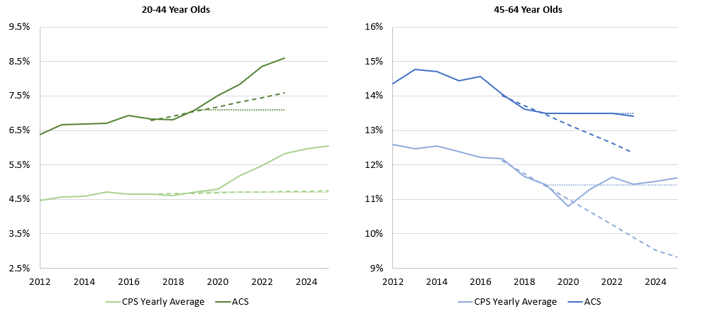
Merge data with CPS annual averages to compare our two data sources.

tables_figures.do

In this do-file, we export our data to Excel (output/spreadsheets/acs_tables_figures.xlsx).

Here’s an example of a graph made by these scripts:

4.2.2 Breakdowns

4.2.2.0.1 demographics.do

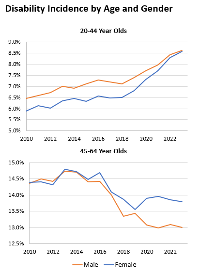
This do-file processes microdata to calculate and export population-weighted disability rates by demographic subgroup over time. It begins by filtering the dataset to include only the non-institutionalized, civilian population age 16 and older, recoding disability variables into binary indicators, and generating subgroup flags for education, race, and gender. It then collapses the data by age and year to compute subgroup-specific disability rates. These rates are adjusted using the 2019 age distribution to produce counterfactual estimates that hold age structure constant across years. The resulting age-adjusted disability rates are calculated for different demographic groups—education, race, and gender—within key age bands (20–44 and 45–64). Finally, the code exports the annual, age-adjusted disability rates for each subgroup and disability type to formatted Excel spreadsheets.

The resulting data is exported to: - breakdowns/demographics/output/spreadsheets/education_tables_figures.xlsx - breakdowns/demographics/output/spreadsheets/race_tables_figures.xlsx - breakdowns/demographics/output/spreadsheets/gender_tables_figures.xlsx

This is entire population weighted (not weighted by subgroup age distributions (out of laziness))

Here is an example of a chart this code generates:

4.2.2.0.2 dot_plots.do

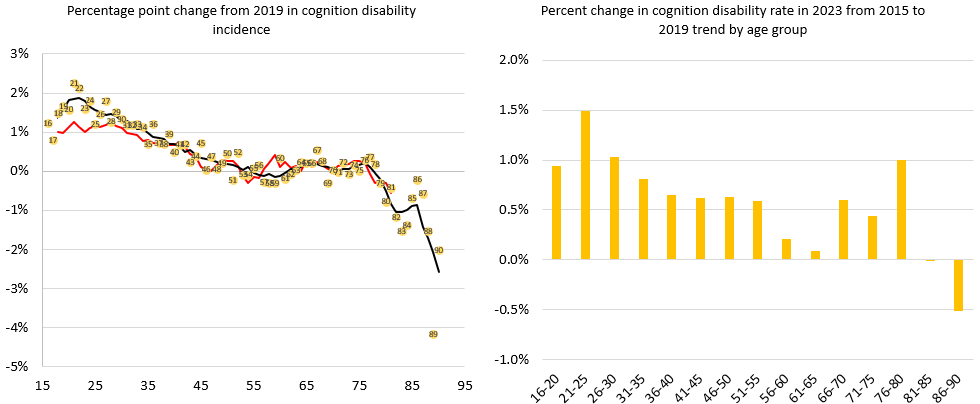
This do-fil processes ACS microdata to measure changes in disability, labor force participation, and telework across age groups over time. It begins by collapsing individual-level data to get age- and year-specific averages for disability incidence and participation. It then computes counterfactual trends—predicted values for 2023 based on linear trends from 2015–2019. Using both observed and counterfactual values, the code calculates percentage and percentage point changes in disability prevalence, participation, and telework for each age and for 5-year age groups. The results are reshaped and exported to a pre-formatted Excel file, with each set of figures saved to a distinct sheet. This setup supports clear visualization of deviations from pre-pandemic trends and enables detailed, age-specific tracking of labor market outcomes among people with disabilities.

The data is exported to output/spreadsheets/acs_dot_plots.xlsx

Here is an example of a graph produced by this code:

4.3 BRFSS

The BRFSS script and file structure is exactly the same as the CPS and ACS. We read in our raw data and clean it in a script called data_clean.do, conduct further analysis in analysis.do, and then output the results to Excel using tables_figures.do.

4.3.0.1 data_clean.do

In this do-file, we read in raw data from the BRFSS and use it to calculate age-adjusted rates of disability incidence, depression, and poor mental health. We also use data from the 2022 and 2023 questionnaires to measure incidence of long COVID for the disability population.

Sections of this code:

Append Yearly Micro Data: In this section, we pull in data from the data_download folder, which contains the raw BRFSS data in SAS format by year. The section does some rudimentary data cleaning (generating variables in the analysis, dropping missing observations, etc.). The code is run in 2-3 year chunks, as they variable codes and variable names changed over the course of the survey, so we cannot clean all survey years in a single loop. For each year, the code will output a temporary file that is stored in data_raw. These temp files are appended to create a large micro data file that aggregates all survey years.
Get Age Shares: In this section, we calculate the 2019 age distribution using the survey weight (called “weight”). This is the weight that was recommended on the BRFSS website. We use these age shares later in the code to age adjust our rates of disability and depression.
Collapse by age and year: Pretty self explantory. We collapse by age and year to get age-specific rates (as a share of the overall population)
Get Counterfactuals: We compare our results to two counterfactuals - the 2019 average rate and the 2017-2019 trend. In this section of code, we perform some additional cleaning and calculate these counterfactuals.
Get Age Distributions: This section of code gets the share of the broader population that falls into each of our age groups of interest. We want to calculate disability incidence, labor force participation, and telework rates for specific age groups. Because these statistics vary significantly across age cohorts, we analyze trends separately for the 20–44, 45–64, and other age groups. To do this, we calculate the proportion of the total population within each age group. For example, to determine the labor force participation rate for the 20–44 age group, we divide the share of people aged 20–44 who are in the labor force by the share of people in that age group. We achieve this later on in the code - this section simply gets us the variables we need to do so. These group-specific rates are also age-adjusted within the cohorts.
Weigh the variables: This is where we actually age adjust our data.

In the last section, we perform some final cleaning to create output/datasets/clean_bynewtime, the dta file that contains monthly, age-adjusted participation and disability rates. We use this dataset to perform some additional analysis in the ‘analysis.do’ script, but the heart of our results are right here in this dataset.

4.3.0.2 analysis.do

In this do-file, we execute further analysis on our cleaned annual data. The sections of this script are fairly self-explanatory. Here they are:

Get the annual disability and depression rates.
Get the annual depression rate.
Get long COVID symptom shares (prevalence of certain symptoms within the long COVID population)
Get long COVID symptoms by disability type.
Get long COVID rates by disability
Get share of the poppulation that HAS EVER HAD long COVID
Get share of the population that is CURRENTLY EXPERIENCING long COVID
Get long covid by age group for the disabled and non-disabled populations.
Get Long covid by age for those with cognition disabilities
Get share of long covid population with a disbaility by disablity type.

4.3.0.3 tables_figures.do

In this section, we export our cleaned data to Excel (output/spreadsheets/brfss_tables_figures.xlsx).

Here is an example of a graph made by this script: