3 Plotting Data

As before, we start by reading the data and packages

library('readr')
library('dplyr')
library('ggplot2')
testdata=read.csv("https://raw.github.com/hdg204/DoctorsAsDataScientists/main/simulated_diabetes_data.csv")

3.1 Introduction to ggplot

In this tutorial we will use a popular R package, ggplot2, to make complex visualisations of data fairly easily. To use ggplot, first you need to tell it what dataframe you’ll be using, and what’s on each axis.

ggplot(data=testdata,aes(x=age))

Figure 3.1: A basic set of axes with bmi on the x axis

This isn’t a very interesting plot, but it creates the canvas for which ggplot can draw on. It knows we’re working with testdata, and it’s put BMI on the x axis.

In the rest of this workshop, we will focus on the different types of figures I find helpful in working with big datasets.

3.2 Bar Charts

We will start with the simple bar chart. First we need to make an axis with something categorical, then we can add a bar chart by literally adding geom_bar()

ggplot(data=testdata, aes(x=gender)) + 
  geom_bar()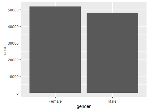

Figure 3.2: A bar chart showing gender distribution

It’s clear, but fairly boring. It also highlights that there is an ‘Other’ category for gender. The aes bit stands for aesthetics and controls a lot about how your graph looks.

ggplot(data=testdata, aes(x=gender,fill=gender)) + 
  geom_bar()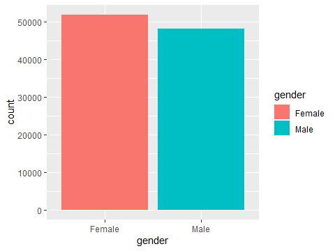

Figure 3.3: A more colourful bar chart

Adding fill=gender tells R that we want the colour every object is filled in to correspond to the gender column. Most people hate that horrible grey background. R has inbuilt themes to modify how the plot looks. I always use theme_bw() or theme_minimal(), but you can make your own stylistic choice.

ggplot(data=testdata, aes(x=gender,fill=gender)) + 
  geom_bar()+
  theme_bw()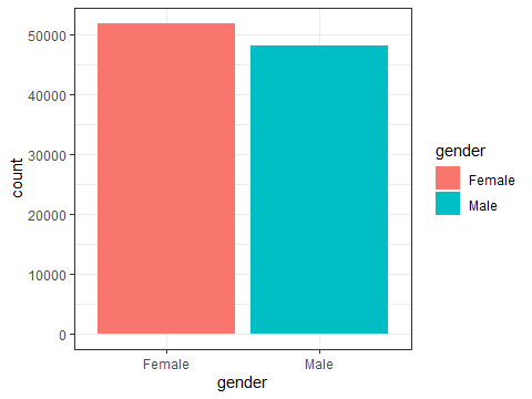

Figure 3.4: A more colourful bar chart

Exercise 1: Produce a coloured bar chart for the smoking_history variable

Exercise 2: Produce a bar chart that has 
smoking history on the x axis but coloured by gender

3.3 Density Plots

Probability density functions show the distribution of your data, a bit like a box plot but in more detail.

ggplot(data=testdata,aes(x=HbA1c_level))+
  geom_density()+
  theme_bw()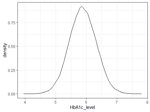

Figure 3.5: A density plot showing the distribution of HbA1c

This shows quite nicely the distribution of HbA1c_level in the data. This can be very useful for highlighting weirdness in your data, and here we see that HbA1c seems to have been rounded, causing odd spikes in the data.

ggplot(data=testdata,aes(x=HbA1c_level,fill=as.factor(diabetes)))+
  geom_density()+
  theme_bw()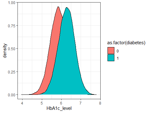

Figure 3.6: A density plot showing the distribution of HbA1c

R needs the as.factor() command for diabetes because it doesn’t know how to turn a numeric variable into a colour. But it’s a bit awkward because one hides the other. We can fix this by adding alpha=0.3 to the geom_density command.

ggplot(data=testdata,aes(x=HbA1c_level,fill=as.factor(diabetes)))+
  geom_density(alpha=0.3)+
  theme_bw()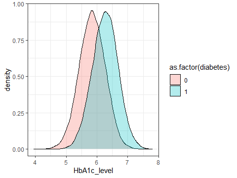

Figure 3.7: A density plot showing the distribution of HbA1c

Exercise 3: Produce a density plot showing the distribution of age by heart disease status

3.4 Scatter Plots

If we want to make a scatter plot, we can add a y axis to the aesthetic. If we want to study the links between bmi and age, we can create an axis

ggplot(data=testdata,aes(x=HbA1c_level,y=bmi))

Figure 3.8: A density plot showing the distribution of HbA1c

We can then add geom_point to this:

ggplot(data=testdata,aes(x=HbA1c_level,y=bmi))+
  geom_point()+
  theme_bw()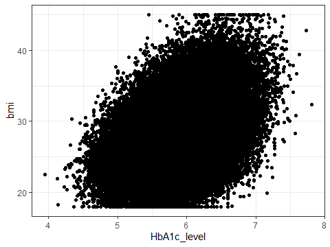

Figure 3.9: A density plot showing the distribution of HbA1c

It’s not the most clear because of how many data points we have, but we can still plot a line through it by adding geom_smooth.

ggplot(data=testdata,aes(x=HbA1c_level,y=bmi))+
    geom_point(alpha=0.01)+
    geom_smooth(size=2)+
    theme_bw()
#> Warning: Using `size` aesthetic for lines was deprecated in ggplot2
#> 3.4.0.
#> i Please use `linewidth` instead.
#> This warning is displayed once every 8 hours.
#> Call `lifecycle::last_lifecycle_warnings()` to see where
#> this warning was generated.
#> `geom_smooth()` using method = 'gam' and formula = 'y ~
#> s(x, bs = "cs")'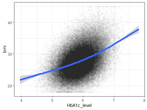

Figure 3.10: A density plot showing the distribution of HbA1c

Here I’ve made the points low alpha and upped the thickness of the line to make it clearer. ggplot’s main strength is the ability to build highly complex graphs with minimal amount of effort. Using almost the same code but adding colour and fill to the aesthetics we can build the following

ggplot(data=testdata,aes(x=HbA1c_level,y=bmi,colour=gender, fill=gender))+
    geom_point(alpha=0.02)+
    geom_smooth(size=2)+
    theme_bw()
#> `geom_smooth()` using method = 'gam' and formula = 'y ~
#> s(x, bs = "cs")'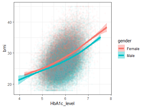

Figure 3.11: A density plot showing the distribution of HbA1c

Note how it knows to plot both the points and the line in the right colour. There’s a lot going on in this plot, but it wasn’t THAT hard to make.

Exercise 4: make a scatterplot of HbA1c level against blood glucose level, 
with the point colour corresponding to diabetes status

3.5 Final Exercise 1

Use mutate to make a new variable overweight, where BMI>25
Use mutate to convert HbA1c to mmol/mol
filter the data to only include people with diabetes
Plot the distribution of HbA1c mmol/mol in people overweight vs not overweight in people with diabetes

3.6 Final Exercise 2

If you got this far, well done. Now, make a thing. I don’t care what it is. Make something new with the data you have.

You’ve got gender, smoking status, hypertension, heart disease, diabetes, bmi, hba1c and blood glucose.

You know how to filter the data and make new variables

You know how to make scatterplots, density plots and bar graphs.

The cheat sheet at https://rstudio.github.io/cheatsheets/data-visualization.pdf has more graph types.

Use your insight as a clinical expert to decide what to look at. Show me if you make anything interesting, or that doesn’t make sense.

2 Dataframes in R