16 Numbers and factors

Seeing numbers in a data file usually seems straightforward. However, erroneous interpretations of numeric information are among the most common errors for inexperienced data analysts.

The two key topics (and corresponding R packages) of this chapter are:

numbers (and their representations)
factors (to handle categorical variables)

Please note: This chapter contains useful notes, but is yet to be finished.

16.1 Introduction

Many people struggle with numeric calculations. However, even people who excel in manipulating numbers tend to overlook their representational properties.

When thinking about the representation of numbers, even simple numbers become surprisingly complicated. This is mostly due to our intimate familarity with particular forms of representation, which are quite arbitrary. When stripping away our implicit assumptions, numbers are quite complex representational constructs.

Main distinctions: Numbers as numeric values vs. as ranks vs. as (categorical) labels.

Example: How tall is someone?

Distinguish between issues of judgment vs. measurement.

When providing a quantitative value, the same measurement can be made (mapped to, represented) on different scales:

size in cm: comparisons between values are scaled (e.g., 20% larger, etc.)
rank within group: comparisons between people are possible, but no longer scaled
categories: can be ordered (small-medium-tall) or unordered (fits vs. does not fit)

Additionally, any height value can be expressed in different ways:

units: 180cm in ft?
accuracy: rounding
number system: “ten” vs. “zehn”, value \(10\) as “1010”” in binary system

Why is this relevant? Distinguish between the meaning and representation of objects:

Different uses of numbers allow different types of calculations and tests.
They should be assigned to different data types.

16.2 Essentials

Important aspects:

Different types of numbers: integers vs. doubles
Numbers as values vs. their name/description/representation (as strings of symbols/digits/numerals).
Some numbers are used to denote categories (identity and difference, but not magnitude/value).

16.3 Numbers

We typically think we know numbers. However, we typically deal with numbers that are represented in a specific numeral system. Our familiarity with specific numeral systems obscures our dependency on arbitrary conventions.

16.3.1 Types of numbers

Different types of numbers (integers vs. doubles):

integers
positive vs. negative
decimals, fractions
real numbers

Consider some oddities:

integers
errors due to floating point (im-)precision

Also relevant: Rules for rounding and scaling numbers.

16.3.2 Representing numbers

When reading a number (like \(123\)), we tend to overlook that this number is represented in a particular notational system. Technically, we need to distinguish between the numeric value \(123\) and the character string of numerical symbols (aka. digits or numerals) “123”.

Generally, numbers are represented according to notational conventions: Strings of dedicated symbols (e.g., Arabic numeral digits 0–9), to be interpreted according to rules (e.g., positional systems require expansion of polynomials).

Overall, our decimal system is a compromise (between more divisible and more unique bases) and a matter of definition. Importantly, our way of representing numbers is subject to two arbitrary conventions:

a positional system with a base value of 10,
representing unit values by the numeral symbols/digits 0–9.

Only changing 2. (by replacing familiar digits with arbitrary symbols) renders simple calculations much more difficult (see letter arithmetic problems).

In the following, we will preserve 2. (the digits and their meaning), but change the base value. This illustrates the difference between numeric value and their symbolic representation (as a string of numeric symbols/digits). (We only cover natural numbers, as they are complicated enough.)

Example

The digits “123” only denote the value of \(123\) in the Hindu-Arabic positional system with a decimal base (i.e., base 10 and numeric symbols 0–9).

Positional notation: Given \(n\) digits \(d_i\) and a base \(b\), a number’s numeric value \(v\) is given by expanding a polynomial sum:

\[v = \sum_{i=1}^{n} {d_i \cdot b^{i-1}}\]

with \(i\) representing each digit’s position (from right to left). Thus, the number \(123\) is a representational shortcut for

\[v = (3 \cdot 10^0) + (2 \cdot 10^1) + (1 \cdot 10^2) = 3 + 20 + 100\]

Representing numbers as base \(b\) positional system

Just like “ten” and “zehn” are two different ways for denoting the same value (\(10\)), we can write a given value in different notations. A simple way of showing this is to use positional number systems with different base values \(b\). As long as \(b \leq 10\), we do not need any new digit symbols (but note that the value of a digit must never exceed the base value).

Note two consequences:

The same symbol string represents different numeric values in different notations:
The digit string “11” happens to represent a value of \(11\) in base-10 notation. However, the same digit string “11” represents a value of \(6\) in base-5 notation, and a value of \(3\) in base-2 notation.
The same numeric value is represented differently in different notations:
A given numeric value of \(11\) is written as “11” in decimal notation, but can alternatively be written as “1011” in base-2, “102” in base-3, and “12” in base-9 notation.

Examples of alternative number systems

Alternatives to the base-10 positional system are not just an academic exercise. See

binary number systems (see Wikipedia: Binary number)
hexadecimal numbers (see Wikipedia: Hexadecimal)

Examples in R

Viewing numbers as symbol strings (of digits): Formatting numbers (e.g., in text or tables)

num_as_char() from the ds4psy package:

ds4psy::num_as_char(1:10, n_pre_dec = 2, n_dec = 0)
#>  [1] "01" "02" "03" "04" "05" "06" "07" "08" "09" "10"

Note the comma() function of the scales package.

base2dec() from the ds4psy package:

ds4psy::base2dec("11")
#> [1] 3
ds4psy::base2dec("111")
#> [1] 7
ds4psy::base2dec("100", base = 5)
#> [1] 25

Demonstration: Show a similation that converts from decimal to another base and back:

Table 16.1: Simulation results of converting decimal numbers (base 10) into another base, and back.
n_org	base	n_base	n_dec
409	15	1C4	409
798	48	GU	798
6340	4	1203010	6340
7179	18	142F	7179
7548	60	25m	7548
6252	6	44540	6252
3759	10	3759	3759
6676	58	1v6	6676
7605	8	16665	7605
3774	58	174	3774
4546	15	1531	4546
542	38	EA	542
9556	8	22524	9556
8973	50	3TN	8973
3390	2	110100111110	3390
5426	53	1nK	5426
4473	54	1Sj	4473
995	57	HQ	995
3116	24	59K	3116
1681	42	e1	1681

See 13 Numbers of r4ds (Wickham, Çetinkaya-Rundel, et al., 2023).

16.3.3 Logical values

The simplest numbers are not even numbers, but the truth values TRUE vs. FALSE.

R uses a convention: In arithmetic expressions, TRUE and FALSE are interpreted as 1 (presence) and 0 (absence), respectively.

This can easily be explored and verified:

TRUE + FALSE
#> [1] 1
TRUE - FALSE
#> [1] 1
TRUE * FALSE
#> [1] 0
TRUE / FALSE
#> [1] Inf

However, the last example shows that we must be careful (e.g., watch out for divisions by zero) should probably not overdo it.

Reasons for this convention: Logical indexing, getting the sums and means of indices. Example:

(age <- sample(1:80, size = 20, replace = TRUE))
#>  [1] 78  9  7  3 43 54 50 11 14 80  2 54 68 50 16 71 67 52 31 28

# Age values of adults:
(age_adults <- age[age >= 18])
#>  [1] 78 43 54 50 80 54 68 50 71 67 52 31 28
length(age_adults)
#> [1] 13

# Arithmetic with logical values:
sum(age >= 18)   # How many adults?
#> [1] 13
mean(age >= 18)  # Proportion of adults?
#> [1] 0.65

Pitfalls of logical values: Using T and F as abbreviations of TRUE and FALSE.

As the documentation of logical() spells out:

TRUE and FALSE are reserved words denoting logical constants in the R language,
whereas T and F are global variables whose initial values set to these.
All four are logical(1) vectors.

Practice

Predict, evaluate, and explain the result of the following expressions:

FALSE / TRUE + 1
FALSE / (TRUE + 1)
FALSE / 100 * TRUE
FALSE + 100 * TRUE
TRUE * 2 * 3 * 4 * 5 * FALSE

16.3.4 Integers

Oddity: See is.integer() vs. is_wholenumber()

16.3.5 Doubles

Pitfalls of floating point numbers:

Oddity: == vs. is.equal()

16.3.6 Precision

An example from Hadley Wickham:

x <- 2     # Assign x to 2
sqrt(x)^2  # should also be 2
#> [1] 2

# But:
x == sqrt(x)^2
#> [1] FALSE

# Even worse:
x <- 1:10
x == sqrt(x)^2
#>  [1]  TRUE FALSE FALSE  TRUE FALSE FALSE FALSE FALSE  TRUE FALSE
# TRUE for 1, 4, 9 (squares of integers), otherwise FALSE

16.3.7 Rounding

Statistical computations are often more precise than what is warranted by the data. For instance, when a sample contains \(N=100\) individuals, some variable (e.g., their height in cm) may average to a numeric value of 178.1234, but if that variable was measured in integers, it does not make sense to provide more than two digits (as an increasing a raw value by \(1\) would change the mean by \(.01\)).

To adjust the precision of a number, we can use round(x) to round a number x to some number of digits.

round(178.1234) # nearest integer (digits = 0)
#> [1] 178
round(178.1234, digits = 1)
#> [1] 178.1
round(178.1234, digits = 2)
#> [1] 178.12

By providing negative values to digits, we can round to the nearest multiple of 10, 100, etc.:

round(178.1234, digits = -1)  # nearest  10
#> [1] 180
round(178.1234, digits = -2)  # nearest 100
#> [1] 200

Most people are surprised by the result of the following rounding operation:

(v <- -5:5 + .50)
#>  [1] -4.5 -3.5 -2.5 -1.5 -0.5  0.5  1.5  2.5  3.5  4.5  5.5
round(v)
#>  [1] -4 -4 -2 -2  0  0  2  2  4  4  6

There is actually a good reason for this seemingly strange behavior: round() uses so-called Banker’s rounding, also known as “round half to even” (and recommended by IEEE / IEC): Any number half way between two integers will be rounded to the even integer. This way, half of the .50 are rounded down, the other half is rounded up, keeping the rounded set unbiased (assuming both cases occur equally often).

If we wanted to force R to always round down or up, we can use the floor() and ceiling() functions, respectively:

floor(v)
#>  [1] -5 -4 -3 -2 -1  0  1  2  3  4  5
ceiling(v)
#>  [1] -4 -3 -2 -1  0  1  2  3  4  5  6

As these functions do not have a digits argument, we can adjust the precision of their results by scaling their arguments:

x <- .345

# Scale to nearest decimal (.10):
.10 * floor(x/.10) 
#> [1] 0.3
.10 * ceiling(x/.10)
#> [1] 0.4

# Scale to nearest percent (.01):
.01 * floor(x/.01) 
#> [1] 0.34
.01 * ceiling(x/.01)
#> [1] 0.35

The same scaling-method allows rounding numbers to the nearest multiple of another number:

# Round to nearest multiple of n:
  5 * round(178.1234/  5)
#> [1] 180
 25 * round(178.1234/ 25)
#> [1] 175
125 * round(178.1234/125)
#> [1] 125

16.3.8 Scaling variables

Skewed data:

hist(v)

Centering and scaling:

hist(scale(v, center = TRUE, scale = FALSE))

hist(scale(v, center = TRUE, scale = TRUE))

Transforming:

hist(log(v))

hist(scale(log(v)))

16.3.9 Using logarithms

Example from McElreath (2018) (Chapter 1, R code 0.3):

The following expressions are mathematically identical

\(p_{1} = \text{log}(.01^{200})\) \(p_{2} = 200 \cdot \text{log}(.01)\)

but R computes two different solutions:

## R code 0.3:
(p_1 <- log(.01^200))
#> [1] -Inf
(p_2 <- 200 * log(.01))
#> [1] -921.034

The value of p_2 (i.e., -921.0340372) is correct. The discrepancy to p_1 is due to rounding, where very small decimal values are rounded to zero and log(0) is -\infty{}. Obviously, such rounding issues can introduce substantial errors. To prevent such errors, expert modelers often perform statistical calculations on the logarithm of probabilities, rather than the probability values themselves.

16.4 Factors

See McNamara & Horton (2018) and 16 Factors of r4ds (Wickham, Çetinkaya-Rundel, et al., 2023).

Encoding categorical data presents specific challenges, but is relevant because many variables are inherently categorical in nature (e.g., gender, blood type, dress size, tax bracket, city, or state). As categorical data can be encoded as text strings (i.e., of type “character” in R) or as numbers, it often remains unnoticed that factors provide an alternative way of dealing with them.

R’s way of encoding categorical data are factors. As many users have a poor understanding of them and may even inadvertently use them, they have a bad reputation. However, they are often useful for representing variables that feature a small and fixed number of categories (e.g., S/M/L; female/male/other) or an ordered number of instances (e.g., days of the week, months). In statistics, factors allow testing for specific effects (e.g., comparing the results of several treatments with those of a control condition).

Categorical data could be represented as numbers, text strings, or as factors.

Example: Gender as “male” vs. “female”. But any survey with more than a few people will require additional categories, like “other” or “do not wish to respond”.

Factors are useful and indispensable (for graphing, statistical analysis), but additional complexity increases chance of unexpected behavior and pitfalls.

Factors are used when variables denote categories or groups. Specific reasons for using factors:

for defining experimental conditions
for ordered categories (e.g., in graphs)

16.4.0.1 Basics

Different factor values are internally represented as integers. This may occasionally seem confusing:

x <- 4:6
c(x)
#> [1] 4 5 6

y <- factor(x)
c(y)
#> [1] 4 5 6
#> Levels: 4 5 6

A neat example of potentially unexpected behavior of factors from McNamara & Horton (2018) (p. 98):

x_org <- c(10, 20, 10, 100, 50)
x_fct <- factor(x_org)
x_fcn <- as.numeric(x_fct)

# Compare (as df):
knitr::kable(data.frame(x_org, x_fct, x_fcn), 
             caption = "Turning a numeric variable into a factor and back...")

Table 16.2: Turning a numeric variable into a factor and back…
x_org	x_fct	x_fcn
10	10	1
20	20	2
10	10	1
100	100	4
50	50	3

When only comparing x_org and x_fct, it seems as converting x_org into a factor had not changed anything. However, when using the base R function as.numeric() on x_fct, we do not recover the original numeric values, but instead yields the values of x_fcn. Instead, we realize that the factor() function mapped the values of x_org to integer values (from 1 to 4) and used the original values as the labels of factor levels. Thus, recovering numeric values from numeric factor variables may yield unexpected results.

A similar surprise may occur when starting with a character object:

as.numeric("txt")
#> [1] NA
as.numeric(factor("txt"))
#> [1] 1

Here, coercing as.numeric("txt") into a missing (NA) value makes perfect sense. However, turning txt into a factor dutifully reports its first level as txt, but internally used the number 1 to encode the first factor level.

Due to unexpected behaviors like this, it recently became unfashionable to automatically convert text variables into factors (e.g., the default read.*() functions have been changed to use stringAsFactors = FALSE). But as many statistical tasks still require index variables (e.g., to denote reference groups), handling factors is still an important and useful skill.

16.4.0.2 Tasks

Structure section by factor-related tasks:

Define a factor with levels: factor()

Example:

wday <- c("Mon", "Tue", "Fri", "Sat", "Thu", "Wed", 
          "Mon", "Sun", "Tue", "Wed", "Thr", "Fri")
mnth <- c("Jan", "May", "Nov", "Apr", "Dec", "Sep", 
          "Jul", "Feb", "Jun", "Oct", "Ian", "Feb")

Problems with using such (character) variables to denote grouped values:

They sort alphabetically, rather than in the way we usually want:

sort(wday)
#>  [1] "Fri" "Fri" "Mon" "Mon" "Sat" "Sun" "Thr" "Thu" "Tue" "Tue" "Wed" "Wed"
sort(mnth)
#>  [1] "Apr" "Dec" "Feb" "Feb" "Ian" "Jan" "Jul" "Jun" "May" "Nov" "Oct" "Sep"

As factors:

# Factor levels:
week_day <-  c("Mon", "Tue", "Wed", "Thu", "Fri", "Sat", "Sun")

# Define factor:
(wday_fct <- factor(wday, levels = week_day))
#>  [1] Mon  Tue  Fri  Sat  Thu  Wed  Mon  Sun  Tue  Wed  <NA> Fri 
#> Levels: Mon Tue Wed Thu Fri Sat Sun

# Similarly (using built-in constant):
(mnth_fct <- factor(mnth, levels = month.abb))
#>  [1] Jan  May  Nov  Apr  Dec  Sep  Jul  Feb  Jun  Oct  <NA> Feb 
#> Levels: Jan Feb Mar Apr May Jun Jul Aug Sep Oct Nov Dec

Now we have:

sort(wday_fct)
#>  [1] Mon Mon Tue Tue Wed Wed Thu Fri Fri Sat Sun
#> Levels: Mon Tue Wed Thu Fri Sat Sun
sort(mnth_fct)
#>  [1] Jan Feb Feb Apr May Jun Jul Sep Oct Nov Dec
#> Levels: Jan Feb Mar Apr May Jun Jul Aug Sep Oct Nov Dec

A 2nd problem is less obvious:
The last sort() silently dropped a vector element, which was NA in our factor definitions (due to a typos in the 2nd last elements). Thus, it may be safer to use the fct() function of the forcats package:

library(forcats)

wday_fct <- forcats::fct(wday, levels = week_day)
#> Error in `forcats::fct()`:
#> ! All values of `x` must appear in `levels` or `na`
#> ℹ Missing level: "Thr"
mnth_fct <- forcats::fct(mnth, levels = month.abb)
#> Error in `forcats::fct()`:
#> ! All values of `x` must appear in `levels` or `na`
#> ℹ Missing level: "Ian"

Using fct() returns an error when a value is not present in levels, thus prevents accidental NA values.

Note

As factors are sorted by the order of their levels, we typically do not need to set ordered = TRUE to create an ordered factor. However, model-fitting functions treat unordered and ordered factors differently.

We can coerce an existing variable into a factor by wrapping it in as.factor().

To illustrate the following steps, we create a factor from a text variable. The factor variable gender_fct distinguishes 4 levels and contains 100 values:

gender_txt <- sample(c("female", "male", "other", "no response"), 
                     size = 100, replace = TRUE, prob = c(.46, .44, .05, .05)) 
gender_fct <- as.factor(gender_txt)

The following functions are useful for inspecting factor variables:

# Inspecting factors:
levels(gender_fct)
#> [1] "female"      "male"        "no response" "other"
summary(gender_fct)
#>      female        male no response       other 
#>          51          38           7           4

Note that summary(x) of a factor x yields the same frequeny table as table(y) of a corresponding non-factor variable y.

Changing the labels of factor levels

Theoretically, changing the labels of factor levels is trivial. We can simply assign different values to the factor’s levels():

levels(gender_fct) <- c("women", "men", "else", "prefer not to say")

However, this is highly risky and error-prone. As a factor’s level labels are usually ordered alphabetically, we just erroneously turned the "other" category into "prefer not to say" and "no response" into "else", rather than vice versa:

summary(gender_fct)
#>             women               men              else prefer not to say 
#>                51                38                 7                 4

A more robust way for changing the factor labels is to use the recode() function of dplyr. By allowing explicit pairs of "old label" = "new label", it is less likely that we will accidentally confuse factor levels:

# Recover our original factor:
gender_fct <- as.factor(gender_txt)  
# levels(gender_fct)
summary(gender_fct)
#>      female        male no response       other 
#>          51          38           7           4

# Recode variable (factor labels): 
gender_fct <- dplyr::recode(gender_fct, 
                            "female" = "women", 
                            "male"   =  "men", 
                            "other"  = "else",
                            "no response" = "prefer not to say")
# levels(gender_fct)
summary(gender_fct)
#>             women               men prefer not to say              else 
#>                51                38                 7                 4

Reorder factor levels

We usually assign the levels of a factor when creating it:

# Create factor (with 4 levels):
gender_fct <- factor(gender_txt, levels = c("female", "male", "no response", "other"))  
summary(gender_fct)
#>      female        male no response       other 
#>          51          38           7           4

If we ever want to change the order of levels, we may be tempted to do the following:

# A BAD approach (NOT to be used):
BAD_fct <- gender_fct  # copy (to keep original factor)
summary(BAD_fct)
#>      female        male no response       other 
#>          51          38           7           4

levels(BAD_fct) <- c("female", "male", "other", "no response")
summary(BAD_fct)
#>      female        male       other no response 
#>          51          38           7           4

Again, this seems trivial, yet introduces an error, as the last two groups were swapped without any warning or error message. Note that the above assignment to levels(BAD) above would be identical to using numerical indexing on the original levels of BAD_fct:

BAD_fct <- gender_fct  # copy (to keep original factor)
levels(BAD_fct) <- levels(BAD_fct)[c(1:2, 4, 3)]
summary(BAD_fct)
#>      female        male       other no response 
#>          51          38           7           4

A legitimate way of re-ordering factor levels in base R would be to re-order them within a factor() function:

# Reorder factor levels (by numerical indexing on existing levels):
new_fct <- factor(gender_fct, levels = levels(gender_fct)[c(1:2, 4, 3)])
summary(new_fct)
#>      female        male       other no response 
#>          51          38           4           7

This changed the order of levels without mixing up the categories and their corresponding counts. (We assigned the result to new_fct to keep the original gender_fct for comparison. If we are sure that we are not messing up, we could directly re-assign the result to gender_fct.)

As this re-leveling within the levels of factor() is a bit tricky, we may be tempted to consider using the relevel() function of the native stats package:

new_fct <- relevel(gender_fct, ref = c("other"))
levels(new_fct)
#> [1] "other"       "female"      "male"        "no response"
summary(new_fct)
#>       other      female        male no response 
#>           4          51          38           7

However, this only allows us to move one level (here "other") forward to use it as the new reference level for statistical comparisons.

A more robust solution for re-ordering factor levels uses the forcats function fct_relevel():

new_fct <- forcats::fct_relevel(gender_fct, "female", "male", "other", "no response")
summary(new_fct)
#>      female        male       other no response 
#>          51          38           4           7

As fct_relevel() retains unmentioned levels behind mentioned ones, the following variant would create the same result:

new_fct <- forcats::fct_relevel(gender_fct, "female", "male", "other")
summary(new_fct)
#>      female        male       other no response 
#>          51          38           4           7

Another useful feature of fct_relevel() is that typos resulting in unknown levels are noted (and no further harm is done, as all unmentioned levels are kept):

new_fct <- forcats::fct_relevel(gender_fct, "male", "female", " other ")
summary(new_fct)
#>        male      female no response       other 
#>          38          51           7           4

Combining several levels into one (both string-like labels and numeric labels)

See 5. Combining several levels into one of McNamara & Horton (2018)

Creating derived factor variables

See 6. Creating derived categorical variables of McNamara & Horton (2018)

Other useful tips

using trimws() to remove leading or trailing whitespace
using unique() for identifying typos and unique factor levels

Note

the forcats package (Wickham, 2023a) is used in Wickham & Grolemund (2017) and Wickham, Çetinkaya-Rundel, et al. (2023).
the last 4 tasks are from (McNamara & Horton, 2018) who contrast fragile and robust solutions for solving these problems.

16.5 Conclusion

Numbers are trickier than we usually think. Not only are there different kinds of numbers, but any given number can be represented in many different ways. Choosing the right kind of number depends on what we want to express by it (i.e., the number’s function or our use of it).

16.5.1 Summary

Key question: Do we mean the number values or their representations?

If value: What do the number values denote (semantics)? What types of numbers and accuracy level is needed?
If representations: In which context are number representations needed? (As numerals or words? Which system? Which accuracy?)

16.5.2 Resources

16.5.2.1 Numbers

16.5.2.2 Factors

Resources for using factors in base R:

McNamara, A., & Horton, N. J. (2018). Wrangling categorical data in R. The American Statistician, 72(1), 97–104. doi: 10.1080/00031305.2017.1356375
Also available at PeerJ.com: https://doi.org/10.7287/peerj.preprints.3163v2
Son Nguyen (2020). Efficient R programming. See Section 3.4 Factors.

Handling factors in tidyverse contexts using the forcats package (Wickham, 2023a):

Chapter 15 Factors of Wickham & Grolemund (2017)
Chapter 16 Factors of Wickham, Çetinkaya-Rundel, et al. (2023)

A good overview of forcats is found on one of the Posit cheatsheets:

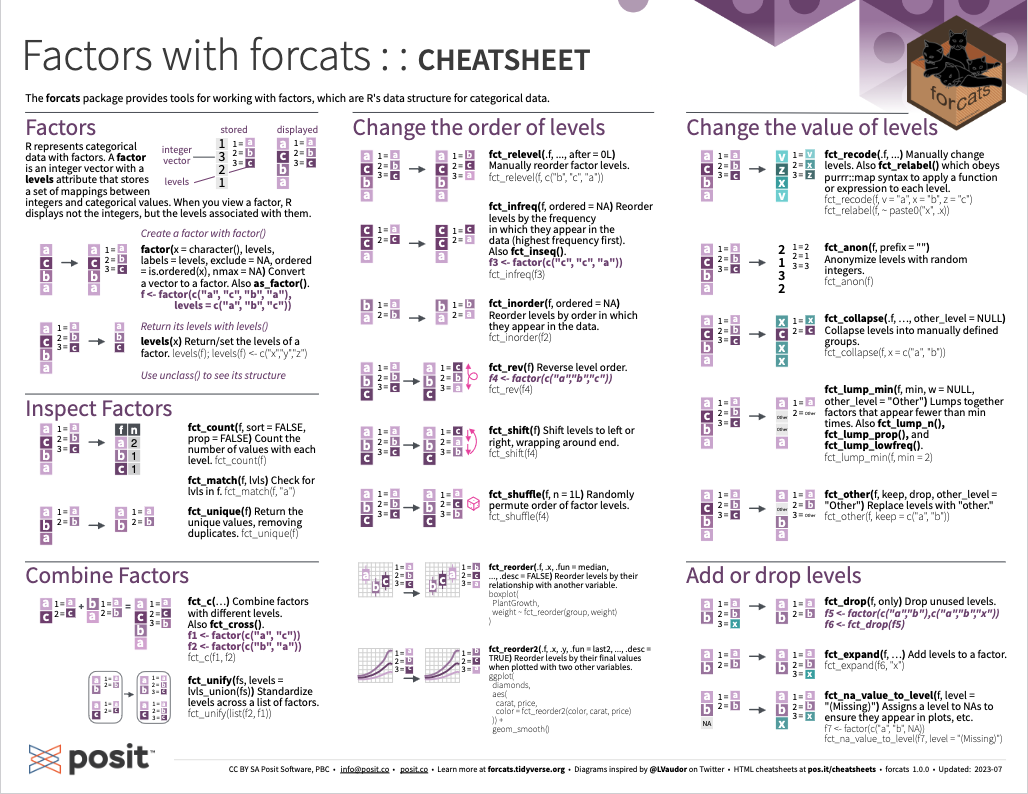
Figure 16.1: Handling factors with forcats from Posit cheatsheets.

16.5.3 Preview

What’s next?

16.6 Exercises

16.6.1 Converting decimal numbers into base N

Create a conversion function dec2base(x, base) that converts a decimal number x into a positional number of different base (with \(2 \leq\) base \(\leq 10\)). Thus, the dec2base() function provides a complement to base2dec() from the i2ds package:

library(i2ds)
base2dec(11, base = 2)
#> [1] 3
dec2base(3,  base = 2)
#> [1] "11"

Use your dec2base() function to compute the following conversions:

dec2base(100, base =  2)
dec2base(100, base =  3)
dec2base(100, base =  5)
dec2base(100, base =  9)
dec2base(100, base = 10)

Create a brief simulation that samples \(N = 20\) random decimal numbers \(x_i\) and base values \(b_i\) \((2 \leq b_i <= 10)\) and shows that

base2dec(dec2base(\(x_i,\ b_i\)),\(b_i\)) ==\(x_i\)

(i.e., converting a numeric value from decimal notation into a number in base \(b_i\) notation, and back into decimal notation yields the original numeric value).

Solution

Table 16.3: Convert integer values from decimal to base notation, and back to decimal notation.
n_org	base	n_base	n_dec	same
6014	7	23351	6014	TRUE
364	8	554	364	TRUE
8030	3	102000102	8030	TRUE
8756	4	2020310	8756	TRUE
5858	7	23036	5858	TRUE
5170	8	12062	5170	TRUE
461	6	2045	461	TRUE
518	10	518	518	TRUE
9642	6	112350	9642	TRUE
7861	9	11704	7861	TRUE
4785	10	4785	4785	TRUE
5514	5	134024	5514	TRUE
4943	8	11517	4943	TRUE
2666	4	221222	2666	TRUE
305	9	368	305	TRUE
7750	3	101122001	7750	TRUE
5471	5	133341	5471	TRUE
5043	7	20463	5043	TRUE
2206	7	6301	2206	TRUE
3280	4	303100	3280	TRUE

16.6.2 Exercise

Part 5: Special data types

17 Text data