Block 1
2025-10-09
General Knowdedge for Instructors
Math 141/142 rely on a homegrown package, USAFACalc, to enhance the course. For Math 141, the relevant features of USAFACalc are entirely convenience features related to graphics. Use them.
Unfortunately, mosaicCalc (what the book relies on), uses an older R graphics system, lattice, which no one uses anymore. I’ve worked hard to build tools that will enable instructors to build professional looking graphics that also match the aesthetic of what we do in class. All of the tools mentioned below work fine with the tools from the book, and support the normal options like add=, col=, lty=, etc.
These are advanced tools, intended for instructors. If you are new to R, I recommend just getting going with R first, and then coming back to this section as you want to build more advanced graphics.
These tools are certainly not required for students to use. They are just for instructors to build good presentations, GR figures, Quiz figures, etc.
It might be tempting to go out to, e.g., Desmos to build figures. Try to avoid that. For one, it is frustrating when all the in-class figures look one way, and then all the figures students can produce look another. Second, many instructors also need some time getting used to our ecosystem. The more time you spend using this ecosystem, the less likely it is that you find something you can’t solve in class.
Each section below gives a quick overview of graphics-type things that you might want to do throughout Math 141. If you run into any problems, contact Joe Eichholz.
All of these tools have documentation that you can find with ?. For instance run the block below for help on mathaxis.on.
Many of these functions take optional arguments with .... If you see ... listed as an option, it is likely that those arguments will be passed through to a lower-level function. For instance, place.text is calling the base text function. Options passed to place.text in the ... space will be passed in to base text. Generally, the help tells you want base functions the ... options will be passed to, so then you can go look at the help for the base function to determine what options are possible.
0.1 Running library
The book states that it is necessary to run
Every time we start R. That is no longer the case. All of these libraries are automatically imported every time you start the Math 141 Project, so the above is unnecessary. It doesn’t hurt anything if you do it, but it is not needed.
0.2 plotFun Options
I’ll point out that there are options for plotFun that help your plots look better, especially when adding multiple plots to the same figure. The lwd option sets the line width. 2 is default. lty sets the line style, you can use “blank”, “solid”, “dashed”, “dotted”, “dotdash”, “longdash”, “twodash” or 0, 1, 2, 3, 4, 5, 6.
plotFun(sin(x)~x, lty="longdash",col="firebrick")
plotFun(cos(x)~x,add=TRUE,lty=5,col="cyan4",lwd=3)
You’ll see me use crazy color names throughout the NTIs. Don’t shy away from them! For one, there are much more appealing looking colors than the default red and blue. Second, I encourage you to let students pick colors for you. Some students get really into finding wierd names, or finding great color combos, or really bad ones. For a few students, this will really help them tune-in.
0.3 grid.on and mathaxis.on
By default plotFun (for plotting functions) and plotPoints for plotting data, do not include traditional “math” axes or a background grid. It can be easy to miss where the axes are. Once you have a figure plotted, you can use mathaxis.on() to turn on the traditional axes, and grid.on to turn on a grid.
plotFun(sin(x)~x, lty="longdash",col="firebrick")
mathaxis.on()
grid.on()
plotFun(cos(x)~x,add=TRUE,lty=5,col="cyan4",lwd=3)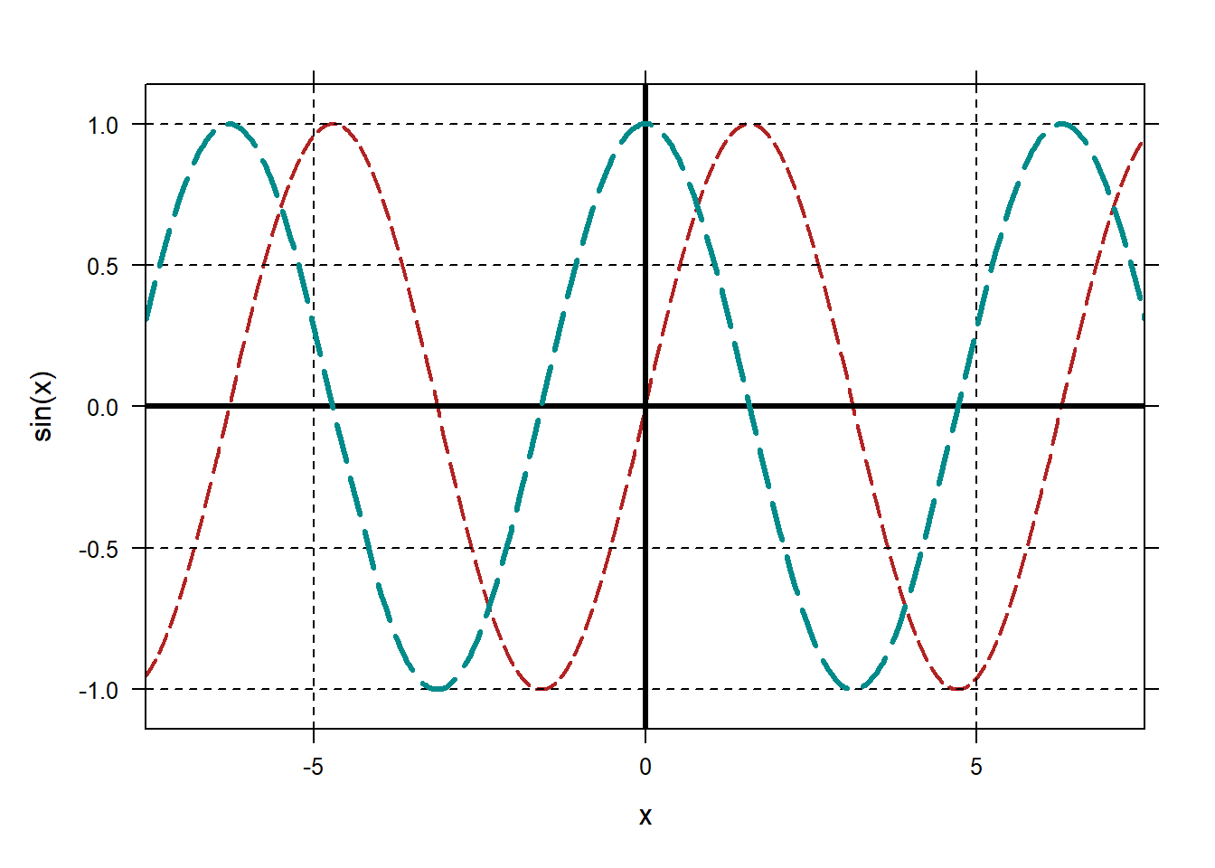
0.4 Adding points to a plot
Sometimes you want to place a dot on a plot, either to highlight a data point or as the base of a vector or whatever. The easiest way to do this is with plotPoints and setting the pch option to 19. pch sets the type of symbol plotted at each data point; you can look up many more. If you need the dot larger or smaller, use the cex option to scale.
Remember that plotPoints takes points in the order y~x.
plotFun(sin(x)~x, lty="longdash",col="firebrick")
mathaxis.on()
plotFun(cos(x)~x,add=TRUE,lty=5,col="cyan4",lwd=3)

plotPoints(1~pi/2,pch=19,col="blueviolet",add=TRUE)
plotPoints(0~pi,pch=19,col="aquamarine2",add=TRUE,cex=2)

plotPoints(c(-1,-1,-1,-1)~c(-pi,-pi/2,pi,3*pi/2),col="chartreuse3",pch=19,add=TRUE,cex=1.3)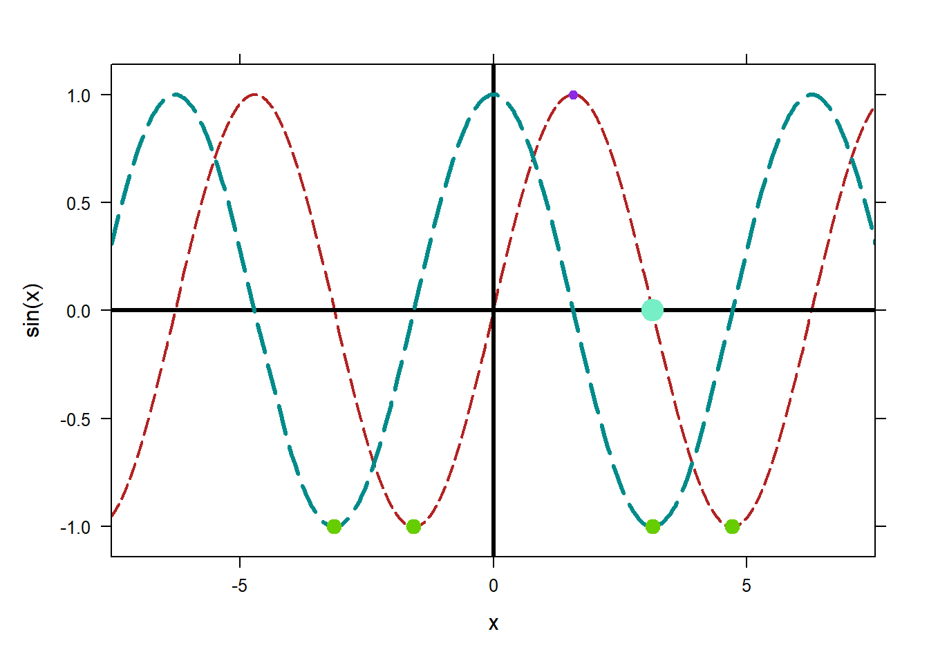
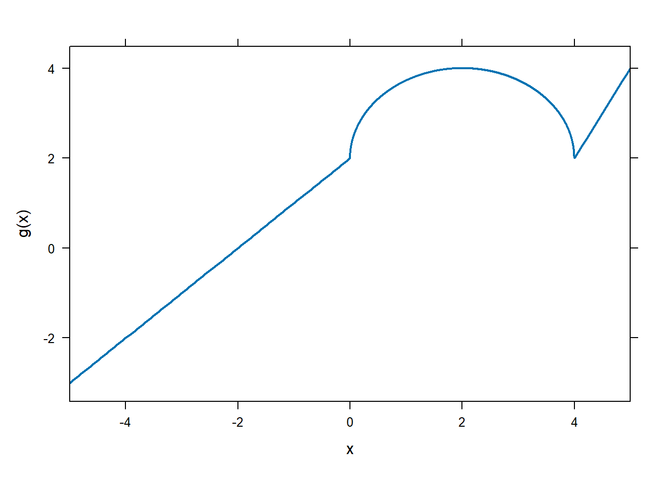
0.5 Piecewise Functions
It’s not so obvious how to make a piecewise defined function with mosaic. To do it, use the R command ifelse combined with makeFun. To define
\[f(x)= \begin{cases} -x^2 &\text{ if } x<0 \\ x^2+4 &\text{ otherwise}\end{cases}\]
as below.
You can nest ifelse to make a more complicated function. For instance
\[g(x)=\begin{cases} x+ 2 &\text{ if } x\le 0\\\sqrt{4-(x-2)^2} &\text{ if } 0<x<4 \\ 2x-6 &\text{ if } 4\le x \end{cases}\]
can be defined as below.
plotFun tries to be clever in order to detect where functions are discontinuous when plotting, and will leave a little gap in the graph around discontinuities. This allows it to do a good job when plotting functions like \(1/x\). However, it often gets tricked by functions which are continuous but not differentiable, like many piecewise functions. In this case, disable the feature by using discontinuity=Inf option.
#This leaves little gaps.
plotFun(g(x)~x,xlim=c(-5,5),lwd=2)
#This looks good.
plotFun(g(x)~x,xlim=c(-5,5),lwd=2,discontinuity = Inf)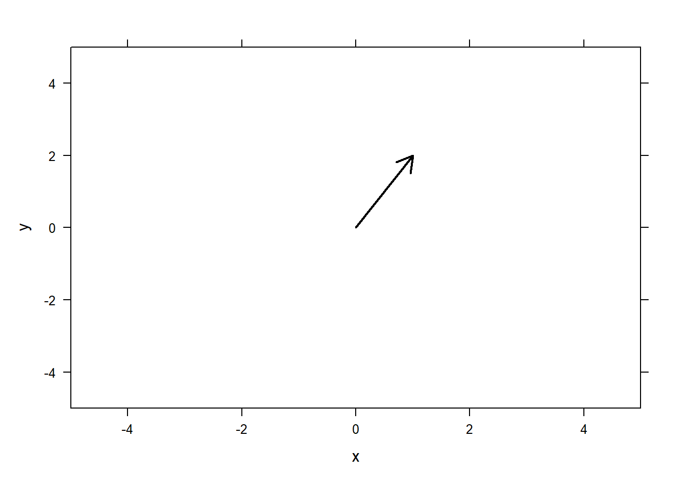
0.6 blank.canvas
Functions mathaxis.on, grid.on, place.text, and place.vector will only add to an existing figure. If you want to make a blank set of axes, or just have one vector hanging out, first create blank canvas with the limits that you want.
 Then, put on what you want.

0.7 place.text
You can place text on your figure using place.text.
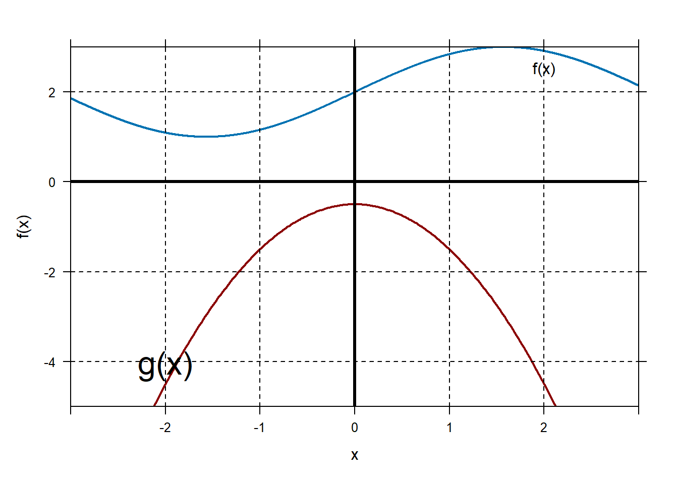
f=makeFun(sin(x)+2~x)
g=makeFun(-x^2-1/2~x)
plotFun(f(x)~x,xlim=c(-3,3),ylim=c(-5,3))
plotFun(g(x)~x,add=TRUE,col="darkred")
grid.on()
mathaxis.on()
place.text("f(x)",x=2.0,y=f(2.0)-0.4)
place.text("g(x)",x=-2,y=g(-2)+0.4,zoom=2)
place.text supports LaTeX. You must replace all backslashes in a normal LaTeX string with double backslashes. The font is the system font, not the normal math font, and sometimes the symbol sizes are a little off, but it is certainly nicer looking than leaving things in plain text. For example:
plotFun(pnorm(x)~x,xlim=c(-3,3),lwd=2)
plotFunFill(pnorm(x)~x,xlim=c(-3,1.5),col='coral2',add=TRUE)
mathaxis.on()
place.text("$x$",1.5,-0.04,zoom=1.3)
place.text("$\\int_{-\\infty}^x \\frac{1}{\\sqrt{2\\pi}} e^{-\\frac{x^2}{2}}\\,dx$",
           0.8,0.3,zoom=1.4)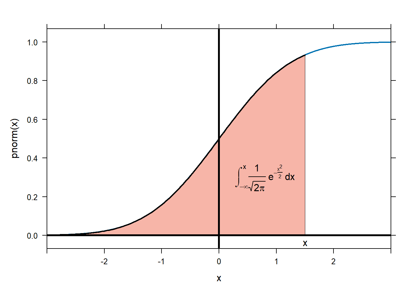
You can change the alignment of text with pos= options. See the base text options with ?text for more detail. For instance, pos=4 means to align on the left.
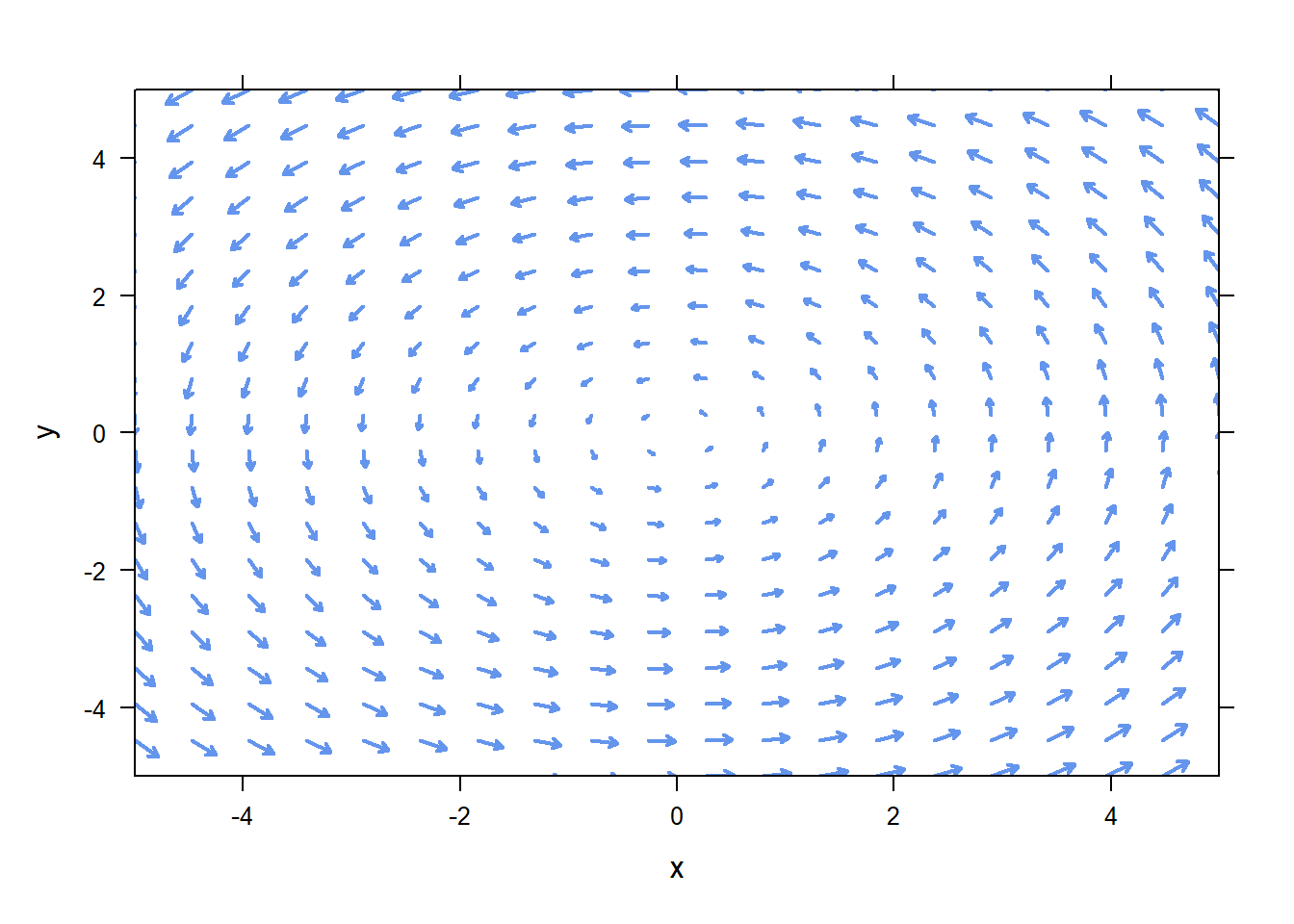
0.8 Plotting Vectors and Vector Fields
The function place.vector will add a single vector to your figure. plotVectorField will plot an entire vector field, with vectors scaled to fit on the figure.
place.vector places a vector emenating from the base you specify (default is (0,0)). It takes the normal col, lwd, and lty options, and it will only add to an existing figure.
plotVectorField plot a vector field.
Vector-valued functions are defined using c. For example, to define the vector-valued function
\[F(x,y)=(-y,x)\]
use
## [1] -3 2Now to plot \(F\).

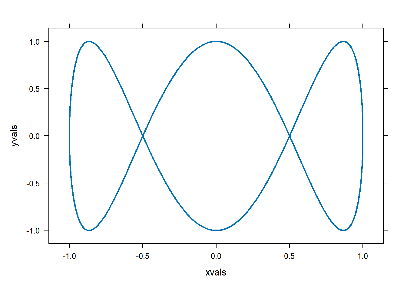
0.9 Plotting parameteric functions
I don’t know that we ever need to do this in Math 141 or Math 142. However, this took me a long time to figure out and we need to document somewhere.
Suppose we want to plot the parametric function \(x(t)=\cos(t)\), \(y(t)=\sin(3t)\). We will need to create data points that are on the parametric curve, and then we’ll use plotPoints to connect them, we’ll use a line style to connect with a line rather than using a bunch of individual points.
x=makeFun(cos(t)~t)
y=makeFun(sin(3*t)~t)
tspan=seq(-10,10,length.out=1000) #create time points at which to evaluate x and y.
xvals=x(tspan)
yvals=y(tspan)

#Plot those points, connect the points with a line.
plotPoints(yvals~xvals,type="l",lwd=2)
0.10 Plotting surfaces
I’ve updated plotFun to produce nicer looking surface plots using the plotly library. It will still produce the old wire mesh plots in the Plots window, but now it will also produce a better looking figure in the Viewer window. It supports the xlim, ylim, and zlim options, as well as a few color options. To produce a surface follow the usage in the book.
To include a color bar, use showcolorscale=TRUE
You can change the color of the plot to a flat built-in R color by specifying the color with col. For some reason, colors ending in numbers don’t work. So firebrick is fine, but firebrick4 does not work. You can also specify a color scheme, like Viridis, Jet, or Blues. You can find a list of color schemes by searching for “plotly color schemes”.