Chapter 1 Sigmoidal Function Reading Supplement
1.1 Part 1
Sigmoidal functions are useful for modeling events with fast initial growth followed by slower growth that tapers off over time. Examples of situations where a sigmoidal function would be suitable include population growth, the spread of a disease, the number of new Twitter users, the number of new iPhone users, etc.
There are many different functions that we could use as our sigmoid function. The phrase “sigmoid” means only that a function has a lower bound, grows slowly at first, then grows quickly, and then levels off to an upper bound. The sigmoid function that we use in this course is:
in this course where \(A\), \(m\), \(s\), and \(v\) are parameters used to specify the shape and position of the function.
The pnorm function is useful for modeling the cumulative size of a population, the cumulative number of sick people, the cumulative number of Twitter users, and the cumulative number of new iPhone users, etc., as a function of time. The pnorm function is related to the normal distribution, i.e., the “bell curve,” that you may be familiar with – the normal distribution represents the frequency of new occurrences over time and typically has a symmetric bell shape as seen in Figure 1. The associated pnorm function is the accumulation of those occurrences over time and has an “S-shape” as seen in Figure 2.


(Note that while we use pnorm to describe a sigmoidal function, we will not be further exploring the normal distribution in this course.)
Before we discuss details of our sigmoid function, it is important to define a few terms. First, when we talk about the minimum or maximum of \(f(x)\) in Figure 2, we are referring to the values that \(f(x)\) approaches as our input variable goes off to negative or positive infinity, respectively. While \(f(x)\) does not actually ever reach a minimum or maximum value, there are clearly lower and upper bounds on the possible output values of \(f(x)\) – these are the what we are referring to as the minimum and maximum of \(f(x)\), respectively.
1.1.1 Function Parameters
The value \(x\) is our input variable.
The value \(m\), referred to as the “mean” or “center” represents the input value for the center output value of our function. In other words, when did we see the biggest increase in active Twitter users, or biggest increase in new disease cases? This value corresponds to the input value for the peak output value of the bell curve in Figure 1. The same input value maps to the middle output value of the S-shaped cumulative function in Figure 2. In other words, half of the growth in the S-shaped function occurs before the input value of \(m\) and the other half occurs after the input value of \(m\). Mathematically speaking, the inverse of the middle output value of the sigmoid function is the mean, i.e., \[f^{-1}\left( \frac{\max(\text{output}) + \min(\text{output})}{2} \right) = m\]
The value \(s\), referred to as the “standard deviation” or “spread”, is a measure of spread or rate. High values of \(s\) imply a slower incline while small values indicate a faster incline. When you plot the pnorm function as in Figure 2, you should note that at the input \(m + s\), the output \(f(m + s)\) is about two-thirds of the way up from the center output, \(f(m)\), to the max output. (This is important for model approximation.)
The value \(A\), referred to as the “amplitude”, is the difference between the maximum and minimum output values (or vice versa if the function is decreasing) and the value for \(v\), referred to as the “vertical shift”, is the minimum output value. Note that the amplitude of a sigmoid function and a sinusoidal function are calculated differently…make sure you know the difference!
Figures 3-6 below illustrate how “\(f(x) = A \cdot \text{pnorm}(x,m,s) + v\)” changes as we modify each of the parameters. Default parameter values are set to \(A = 1\), \(m = 0\), \(s = 1\), and \(v = 0\).


1.2 Part 2
We are interested in fitting sigmoid models to real-world data so that we can conjecture output values for various inputs (within the bounds of the input values used to build the model) and, eventually, use the tools of calculus to analyze the fitted model. In order to use the fitModel function in R to fit a pnorm function to a dataset, we must provide estimates for each of the parameters within the \(f(x) = A \cdot \text{pnorm}(x,m,s) + v\) model in a similar way to how we did so when fitting a sinusoidal model to a dataset.
fitModel function in R. Figure 7 below gives an example of how to generate parameter estimates using a graph of S-shaped data.
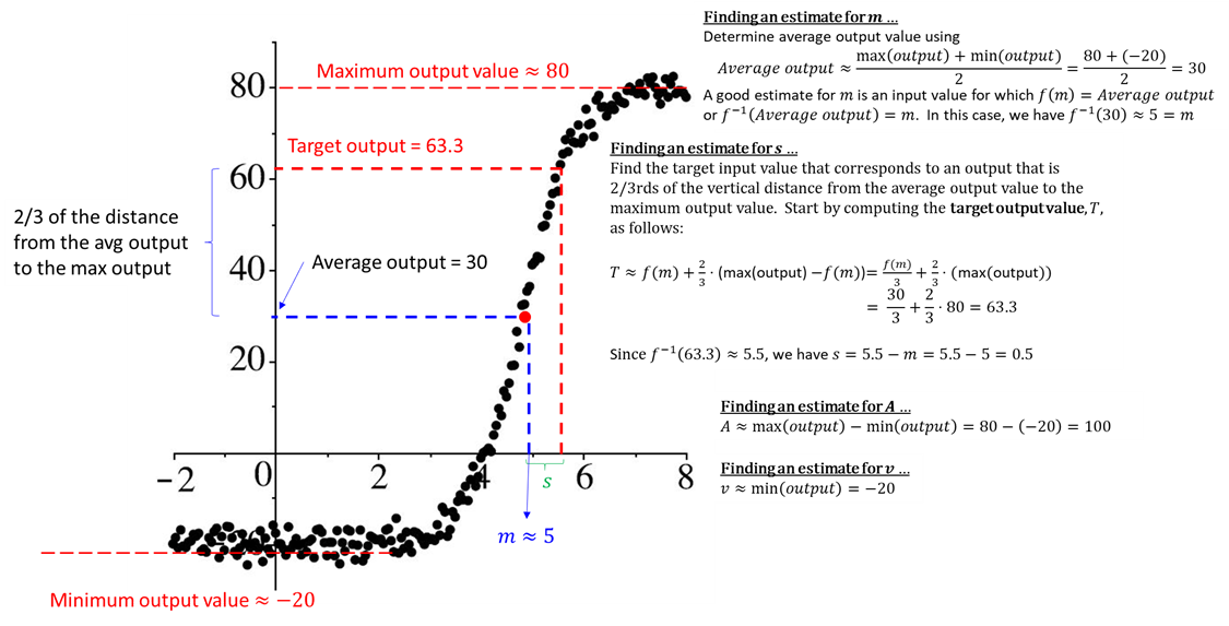
Figure 1.1: Figure 7: Estimating sigmoid parameters from data
Once we have estimates for the sigmoid function parameters, we can use the fitModel command in R to find the best fit model for the dataset. Unfortunately, the graph above did not come with an associated dataset, so we are going to use an MMAC dataset in R (YellowCards) to build another example. This dataset contains the number of yellow cards given per men’s World Cup tournament from 1970 to 2010 – the data is roughly S-shaped and appears to have a clear lower and upper bound. While it does not entirely make sense why the number of yellow cards given per World Cup tournament would follow a sigmoid function pattern, it is not entirely unreasonable to expect a sharp rise in the number of cards given followed by a leveling-out period as it becomes logistically infeasible to give out significantly more yellow cards without completely disrupting tournament play. (If this explanation is less-than satisfying, just know that the YellowCards dataset is referenced in Chapter 2.5 which is called “Modeling with Sigmoidal Functions.”) If we graph this dataset in R, we can use the graph to estimate parameters for a sigmoidal function as seen in Figure 8.

Now that we have estimates for \(A\), \(m\), \(s\), and \(v\) and a dataset to work with, we can use R to find the best fit model. First, let’s graph our estimated model on the data to get a sense for how our estimated function looks.
Aest=250
vest=50
sest=8
mest=1990

plotPoints(Cards~Year,data=YellowCards)
plotFun(250*pnorm(x,1990,8)+50~x,add=TRUE,col="firebrick")
Our estimates seem to produce a fairly good model for this data; however, we can use R to find a better model using the fitModel function. To do this, we execute the following command: (Note that we defined the parameters Aest, mest, sest, and vest in the code shown in Figure 9 for our estimates of each our parameters.)
bestSigFit = fitModel(Cards ~ A*pnorm(Year, m, s) + v,
                      data = YellowCards,
                      start = list(A = Aest, m = mest, s = sest, v = vest))
We can view the best fit model parameters and graph the model with our previous results as follows:

Notice that the best fit model is slightly different than what we estimated. We will discuss what it means for a model to be “best fit” more in the next block. For now, just know that the fitModel command will give us the model that best fits our data as long as we give the function a reasonable set of estimates for the parameter values. If we do not seed the function with a set of reasonable estimates, the fitModel command may not find the best fit model. For example, if we had used a poor estimate for the amplitude (or just fat-fingered in the wrong value), we might get the following results: (Note that I changed the estimate for “A” to “25” versus “250” and left the other estimates the same as before.)
bestSigFit = fitModel(Cards ~ A*pnorm(Year, m, s) + v,
                      data = YellowCards,
                      start = list(A = 25, m = mest, s = sest, v = vest))
## Warning in pnorm(Year, m, s): NaNs produced## Error in numericDeriv(form[[3L]], names(ind), env, central = nDcentral): Missing value or an infinity produced when evaluating the modelThis error message essentially means that at least one of your initial parameter estimates is not suitably accurate and the fitModel function was unable to converge on the best fit model. In this case, you should double check your estimates to make sure you estimated and typed them in correctly. Good luck!