Chapter 3 Gender and Education Inequlaity in COVID19
3.1 data step 1
library(tidyverse)
library(htmlTable)
library(readxl)
library(ggrepel)
#library(doMC)
#registerDoMC(31)
library(data.table)
library(DT)
library(plotly)
library(readr)
3.2 load data of Int and Kr
data import of international and korea
getwd()## [1] "/home/sehnr/projects/covid_int/occup_health"#new laura data Dec 2020
#korea data
#write_csv(covid_data, '/home/sehnr/projects/covid_int/data/covid.csv')
covid = read_csv('/home/sehnr/projects/covid_int/data/covid.csv')
kr_d <- read_xlsx('data/kr_data.XLSX', sheet = 1)
#international data
cbook <- read_xlsx('data/code_book.xlsx')country_lkup <- data.frame(country = c(1, 16, 31, 36,65, 75, 79, 104, 136, 137, 143, 156, 168, 172, 173, 179, 183, 192),
country_c = c(
"USA", "Belarus", "Canada", "China",
"German", "Hong Kong", "Indonesia",
"Malaysia", "Philipines", "Poland",
"Rusia", "Singapore", "Sweden",
"Thailand", "Taiwan", "Turkey",
"Ukraina", "Vietnam"
))overview of codebook
cbook %>% datatable() 'country' = Q2,
'gender' = Q10,
'Birthyear' = Q79,
'Education' = Q80,
'Employment' = Q94,
'today_dep_anxi' = Q41_5, # for korea 'Q22_5'
'emotion_dpressed' = Q36_2, # for korea Q18_2 : how much...
'emotion_anxiety' = Q36_3, # for Korea Q18_3Korea Data step
kr_d1 <- kr_d %>%
      select('IDnum' = No, 'age' = SQ2, 'gender' = SQ1, 'Education'  = DQ1,
             contains('DQ2'), # employment status
             'EmoDep'  = Q18_2, # for int Q36_2 how much have you feeling
             'EmoAnx'  = Q18_3, # for int Q36_3
             'ChrDep'  = Q21_10, # for int Q40_17
             'ChrAnx'  = Q21_11, # for int Q40_18
             'ToDepAnx'= Q22_5, # for int Q41_5,
             'dfLossJob' = Q10_10, # for int Q26_9,
             'dfReduIcm' = Q10_3, # for int Q26_3,
             'dfIncAnx'  = Q10_5 # for int Q26_5
             ) %>%
  mutate(country = 200, country_c = 'Korea') %>%
  map_if(is.numeric, ~ifelse(is.na(.x), 0, .x) ) %>%
 as.data.frame()

#colnames(kr_d1) <- colnames(kr_d1) %>%
#                       str_replace(., "DQ2_", "em")
colnames(kr_d1)
## [1] "IDnum" "age" "gender" "Education" "DQ2_1" "DQ2_2"
## [7] "DQ2_3" "DQ2_4" "DQ2_5" "DQ2_6" "DQ2_7" "DQ2_8"
## [13] "DQ2_9" "DQ2_10" "DQ2_11" "DQ2_12" "DQ2_13" "DQ2_14"
## [19] "EmoDep" "EmoAnx" "ChrDep" "ChrAnx" "ToDepAnx" "dfLossJob"
## [25] "dfReduIcm" "dfIncAnx" "country" "country_c"international Data step
int_d1 <- covid %>%
      mutate('age' = 2020 - Q79) %>%
     mutate(IDnum = row_number()) %>%
      select(IDnum,
             'age',
             'gender' = Q10, 'Education'  = Q80,
             contains('Q94'), # employment status
             'EmoDep'  = Q36_2,
             'EmoAnx'  = Q36_3,
             'ChrDep'  = Q40_17,
             'ChrAnx'  = Q40_18,
             'ToDepAnx'= Q41_5,
             'dfLossJob' = Q26_9,
             'dfReduIcm' = Q26_3,
             'dfIncAnx'  = Q26_5,
             'country' = Q2
             ) %>%

   left_join(country_lkup,  by = c('country')) %>%
   select(-Q94_18, -Q94_19)
Harmonizing Variable name to int
em_lkup = tibble(
  'kr' = c('DQ2_1', 'DQ2_2', 'DQ2_3', 'DQ2_4', 'DQ2_5', 'DQ2_6', 'DQ2_7',
           'DQ2_8','DQ2_9','DQ2_10','DQ2_11','DQ2_12','DQ2_13','DQ2_14'),
  'int' =c('Q94_9', 'Q94_2',    'Q94_3',    'Q94_4',    'Q94_7',    'Q94_8',    'Q94_5',    'Q94_12',   'Q94_14',   'Q94_15',   'Q94_1',    'Q94_6',    'Q94_16',   'Q94_17')

)

kr_d2<- kr_d1 %>%
plyr::rename(setNames(em_lkup$int, em_lkup$kr)) # change kr vairalbe names to int variabl names.

colnames(kr_d2)   == colnames(int_d1)
## [1] TRUE TRUE TRUE TRUE TRUE TRUE TRUE TRUE TRUE TRUE TRUE TRUE TRUE TRUE TRUE
## [16] TRUE TRUE TRUE TRUE TRUE TRUE TRUE TRUE TRUE TRUE TRUE TRUE TRUE3.3 data merge
mm <- rbind(int_d1, kr_d2)
nrow(mm)
## [1] 19270mm <- mm %>% na.omit(age)
nrow(mm)## [1] 16942data mutate
krtoint = function(x) {
  x = ifelse(x<4, x+4, x)
}
logictozero= function(x){
  x = as.numeric(x != 0)
}
mm1 <-mm %>%
  filter(age >20 & age <65) %>%
  filter(gender %in% c(1, 2))

mm12<- mm1 %>%
  mutate(EmoDep =krtoint(EmoDep),
         EmoAnx =krtoint(EmoAnx),
         ToDepAnx=ifelse(ToDepAnx == 3, 1, 0)) %>%
  select(-c('ChrDep', 'ChrAnx', 'dfLossJob','dfReduIcm','dfIncAnx' ))

mm13 <- mm1 %>%
  select(c('ChrDep', 'ChrAnx', 'dfLossJob','dfReduIcm','dfIncAnx' )) %>%
  lapply(., logictozero) %>%
  data.frame()

mm2 <- cbind(mm12, mm13)


mm3 <- mm2 %>%
  mutate(EcLoss       = ifelse(Q94_3 !=0 | Q94_4!=0, 1, 0)) %>%
  mutate(EcLossUnSafe = ifelse(Q94_4!=0, 1, 0)) %>%
  mutate(agegp = cut(age, breaks = c(-Inf, (5:13)*5, +Inf))) %>%
  mutate(agegp2 = as.numeric(agegp)) %>%
  mutate(genders = ifelse(gender ==1, 'Men', 'Women')) %>%
  mutate(Edugp = factor(Education, levels = c(1, 2, 3, 4, 5, 6),
                        labels = c("Middle or less", "High", "Colleage",
                                   "University", "Graduate Sc", "Doctoral or more"))) %>%
  mutate(EcLossAll = EcLoss + dfLossJob ) %>%
  mutate(TotalDepAnx= as.numeric((as.numeric(EmoDep ==7) + as.numeric(EmoAnx ==7))) !=0)
create basic matrix for visualization (NA as zero)
mm4 <- mm3 %>%
    mutate(agegp3 = ifelse(age <=40, '≤40', '>40')) %>%
  mutate(agegp3 = factor(agegp3, levels=c('≤40', '>40'))) %>%

  filter(Education %in% c(1:6)) %>%
 mutate(edugp = ifelse(Education %in% c(1, 2), 1, # high shcool or less
                        ifelse(Education %in% c(3),2, # colleage
                               ifelse(Education %in% c(4), 3, 4)))) %>% # university (5, 6) Graduate school
 mutate(edugp2 = ifelse(Education %in% c(1, 2, 3), 1, 2)) %>%
 mutate(EcLossAllgp = ifelse(EcLossAll ==0, 0, 1)) #%>%
#filter(!country %in% c(16, 173))

bm1<-crossing(
    'genders'=unique(mm4$genders),
    'country_c'=unique(mm4$country_c),
    'edugp'=unique(mm4$edugp),
    'edugp2'=unique(mm4$edugp2),
    'agegp2'=unique(mm4$agegp2),
    'agegp3'=unique(mm4$agegp3),
    'EcLossAllgp'=unique(mm4$EcLossAllgp),
    'TotalDepAnx' = unique(mm4$TotalDepAnx)
)
3.4 Data analysis start
3.4.1 job loss due to covid vary by country
basic static for job loss prevalance across coutnry and genders.
mm4 %>%
  group_by(country_c, genders) %>%
  count(EcLoss) %>%
  mutate(prob = n/sum(n)) %>%
  filter(EcLoss == 1 ) %>%
  ggplot(aes(x = genders, y = prob, fill = genders)) +
  geom_bar(stat = "identity")+
  ylab("job loss due to COVID19")+
  scale_y_continuous(labels = function(x) paste0(x*100, "%"))+
  facet_wrap(country_c ~., nrow = 5)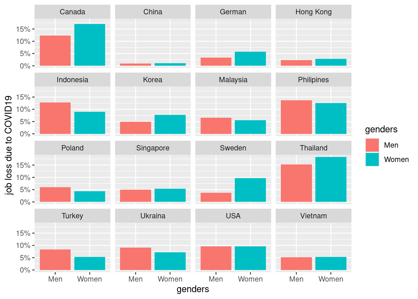
3.4.2 final job loss status
We decide EcoLossAll as representative valu of job loss.
figure using of EcoLossAll
mm4 %>%
  #filter(!country %in% c(16, 173)) %>%
  group_by(country_c, genders, agegp2) %>%
  count(EcLossAll) %>%
  mutate(prob = n/sum(n)) %>%
  filter(EcLossAll == 1) %>%
  ggplot(aes(x = agegp2, y = prob, color = genders)) +
  geom_point(aes(size = n), alpha = 0.2, show.legend = FALSE) +
  geom_smooth(method = 'loess', span =0.9,  se=FALSE) +
   ylab("EcoLossAll due to COVID19")+
    scale_y_continuous(labels = function(x) paste0(x*100, "%"))+
  theme_minimal() +
  xlab("Age (size = number of respondents)") +
  labs(color = "Gender") +
  facet_wrap(country_c~., nrow =3)
## `geom_smooth()` using formula 'y ~ x'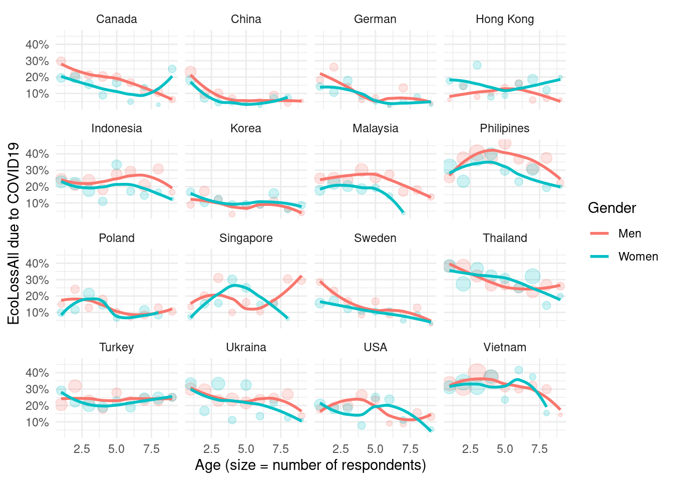
3.4.3 Depression status according job loss status
final psychological symptoms
mm4 %>%
  #filter(!country %in% c(16, 173)) %>%
  group_by(country_c, genders, agegp2) %>%
  count(TotalDepAnx) %>%
  mutate(prob = n/sum(n)) %>%
  filter(TotalDepAnx == 1) %>%
  ggplot(aes(x = agegp2, y = prob, color = genders)) +
  geom_point(aes(size = n), alpha = 0.2, show.legend = FALSE) +
  geom_smooth(method = 'loess', span =0.9,  se=FALSE) +
   ylab("TotalDepAnx due to COVID19")+
    scale_y_continuous(labels = function(x) paste0(x*100, "%"))+
  theme_minimal() +
  xlab("Age") +
  labs(color = "Gender") +
  facet_wrap(country_c~., nrow =4)
## `geom_smooth()` using formula 'y ~ x'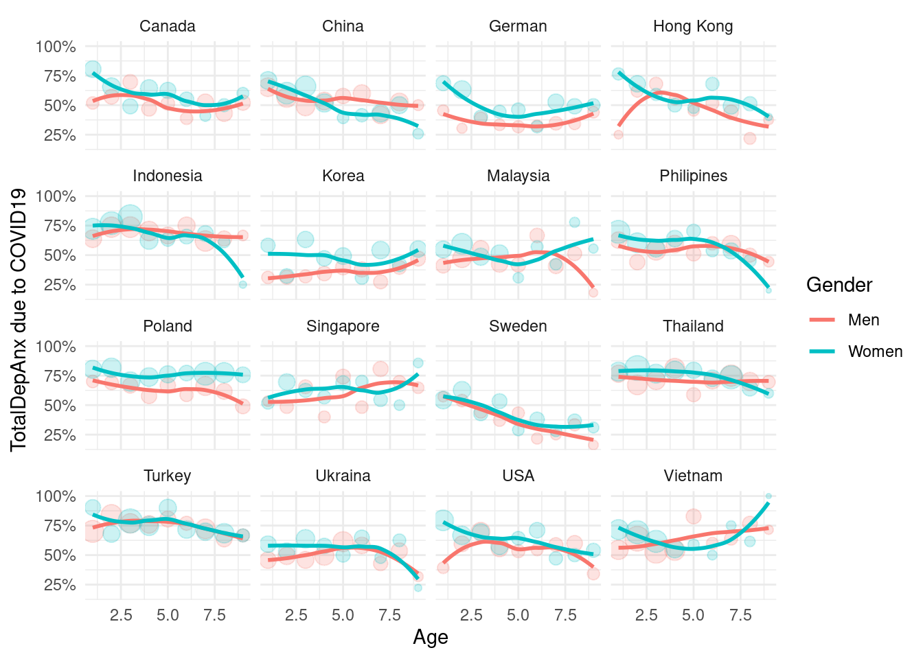
3.5 association
(ref: https://cran.r-project.org/web/packages/sjPlot/vignettes/tab_model_estimates.html)
if (!require('sjPlot')) install.packages('sjPlot')
if (!require('sjmisc')) install.packages('sjmisc')
if (!require('sjlabelled')) install.packages('sjlabelled')
library(sjPlot);library(sjmisc);library(sjlabelled)
mm4 %>%
group_by(country_c) %>%
count()## # A tibble: 17 x 2
## # Groups: country_c [17]
## country_c n
## <chr> <int>
## 1 Canada 769
## 2 China 1197
## 3 German 699
## 4 Hong Kong 530
## 5 Indonesia 1003
## 6 Korea 1032
## 7 Malaysia 873
## 8 Philipines 908
## 9 Poland 888
## 10 Singapore 477
## 11 Sweden 723
## 12 Taiwan 694
## 13 Thailand 1030
## 14 Turkey 973
## 15 Ukraina 927
## 16 USA 780
## 17 Vietnam 991mod1 = mm4 %>%
glm(family = binomial,
formula = TotalDepAnx ~ EcLossAll)
mod2 = mm4 %>%
glm(family = binomial,
formula = TotalDepAnx ~ EcLossAll + age + gender + edugp)
mod3 = mm4 %>%
glm(family = binomial,
formula = TotalDepAnx ~ EcLossAll + age + gender + edugp +
relevel(as.factor(country_c), ref = 'Taiwan') )tab_model(mod1, mod2, mod3)## Profiled confidence intervals may take longer time to compute. Use 'df_method="wald"' for faster computation of CIs.
## Profiled confidence intervals may take longer time to compute. Use 'df_method="wald"' for faster computation of CIs.
## Profiled confidence intervals may take longer time to compute. Use 'df_method="wald"' for faster computation of CIs.| TotalDepAnx | TotalDepAnx | TotalDepAnx | |||||||
|---|---|---|---|---|---|---|---|---|---|
| Predictors | Odds Ratios | CI | p | Odds Ratios | CI | p | Odds Ratios | CI | p |
| (Intercept) | 1.33 | 1.28 – 1.38 | <0.001 | 1.01 | 0.83 – 1.22 | 0.943 | 0.63 | 0.49 – 0.81 | <0.001 |
| EcLossAll | 1.42 | 1.32 – 1.51 | <0.001 | 1.40 | 1.31 – 1.50 | <0.001 | 1.35 | 1.26 – 1.45 | <0.001 |
| age | 0.99 | 0.99 – 0.99 | <0.001 | 0.99 | 0.99 – 0.99 | <0.001 | |||
| gender | 1.33 | 1.24 – 1.42 | <0.001 | 1.34 | 1.25 – 1.43 | <0.001 | |||
| edugp | 1.09 | 1.05 – 1.13 | <0.001 | 1.10 | 1.06 – 1.14 | <0.001 | |||
|
relevel(country_c, ref = “Taiwan”)Canada |
1.39 | 1.12 – 1.71 | 0.002 | ||||||
|
relevel(country_c, ref = “Taiwan”)China |
1.31 | 1.09 – 1.59 | 0.005 | ||||||
|
relevel(country_c, ref = “Taiwan”)German |
0.91 | 0.74 – 1.13 | 0.411 | ||||||
|
relevel(country_c, ref = “Taiwan”)Hong Kong |
1.22 | 0.97 – 1.53 | 0.087 | ||||||
|
relevel(country_c, ref = “Taiwan”)Indonesia |
2.52 | 2.06 – 3.09 | <0.001 | ||||||
|
relevel(country_c, ref = “Taiwan”)Korea |
2.73 | 2.23 – 3.33 | <0.001 | ||||||
|
relevel(country_c, ref = “Taiwan”)Malaysia |
1.01 | 0.83 – 1.24 | 0.905 | ||||||
|
relevel(country_c, ref = “Taiwan”)Philipines |
1.36 | 1.11 – 1.66 | 0.003 | ||||||
|
relevel(country_c, ref = “Taiwan”)Poland |
2.88 | 2.34 – 3.56 | <0.001 | ||||||
|
relevel(country_c, ref = “Taiwan”)Singapore |
1.71 | 1.35 – 2.18 | <0.001 | ||||||
|
relevel(country_c, ref = “Taiwan”)Sweden |
0.78 | 0.63 – 0.97 | 0.027 | ||||||
|
relevel(country_c, ref = “Taiwan”)Thailand |
3.02 | 2.46 – 3.71 | <0.001 | ||||||
|
relevel(country_c, ref = “Taiwan”)Turkey |
3.29 | 2.67 – 4.06 | <0.001 | ||||||
|
relevel(country_c, ref = “Taiwan”)Ukraina |
1.16 | 0.95 – 1.42 | 0.147 | ||||||
|
relevel(country_c, ref = “Taiwan”)USA |
1.67 | 1.36 – 2.06 | <0.001 | ||||||
|
relevel(country_c, ref = “Taiwan”)Vietnam |
1.63 | 1.34 – 2.00 | <0.001 | ||||||
| Observations | 14494 | 14494 | 14494 | ||||||
| R2 Tjur | 0.007 | 0.018 | 0.061 | ||||||
summay stat of each models.
mm4 %>%
  group_by(edugp, country_c, genders) %>%
  count(EcLossAllgp ) %>%
  mutate(prob = n/sum(n)) %>%
  filter(EcLossAllgp  == 1) %>%
  ggplot(aes(x = edugp, y = prob, color = genders)) +
  geom_smooth() +

  scale_x_continuous(labels=c("1" = "≤H", "2" = "C",
                            "3" = "U", "4" = "G")) +
  theme_minimal() +
  ylab("Economic Loss due to COVID19") +
  xlab("H = high school, C = colleage") +
  facet_wrap(country_c ~., nrow = 4)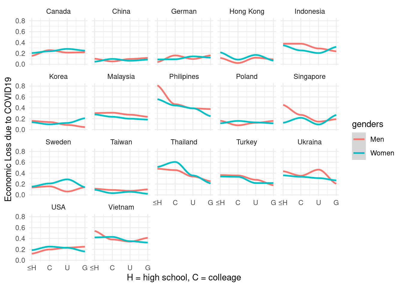
mm5 <- mm4 %>%
  mutate(EcLoss = ifelse(EcLossAllgp ==0, 'Active', 'Loss')) %>%
  mutate(Edgp = ifelse(edugp2 ==1, 'Low', 'High')) %>%
  mutate(int = ifelse( EcLoss == 'Active' & Edgp == 'High', 1,
                       ifelse(EcLoss == 'Active' & Edgp == 'Low',2,
                              ifelse(EcLoss == 'Loss' & Edgp == 'High',3,4
                              )))) %>%
   mutate(int2 = ifelse( Edgp == 'High' & EcLoss == 'Active', 1,
                       ifelse(Edgp == 'High' & EcLoss == 'Loss',2,
                              ifelse(Edgp == 'Low' & EcLoss == 'Active',3,4
                              ))))
men = mm5 %>% filter(genders == 'Men')
women = mm5 %>% filter(genders == 'Women')
mod_men_int1 = men %>%
  glm(family   = binomial,
      formula = TotalDepAnx ~ as.factor(int2))
mod_men_int2 = men %>%
  glm(family   = binomial,
      formula = TotalDepAnx ~ as.factor(int2) +age )
mod_men_int3 = men %>%
  glm(family   = binomial,
      formula = TotalDepAnx ~ as.factor(int2) + age  +country_c)
mod_women_int1 = women %>%
  glm(family   = binomial,
      formula = TotalDepAnx ~ as.factor(int2))
mod_women_int2 = women %>%
  glm(family   = binomial,
      formula = TotalDepAnx ~ as.factor(int2) +age )
mod_women_int3 = women %>%
  glm(family   = binomial,
formula = TotalDepAnx ~ as.factor(int2) + age +country_c) summary(mod_men_int1)$coefficient[1:4, ]## Estimate Std. Error z value Pr(>|z|)
## (Intercept) 0.2135969 0.03276340 6.519376 7.060047e-11
## as.factor(int2)2 0.4013747 0.07168330 5.599278 2.152462e-08
## as.factor(int2)3 -0.2683286 0.05751959 -4.664996 3.086231e-06
## as.factor(int2)4 0.3313844 0.08813473 3.759976 1.699299e-04summary(mod_men_int2)$coefficient[1:4, ]## Estimate Std. Error z value Pr(>|z|)
## (Intercept) 0.4496790 0.08817876 5.099629 3.403196e-07
## as.factor(int2)2 0.3872681 0.07187575 5.388022 7.123728e-08
## as.factor(int2)3 -0.2547112 0.05774117 -4.411259 1.027715e-05
## as.factor(int2)4 0.3166842 0.08832463 3.585458 3.364875e-04summary(mod_men_int3)$coefficient[1:4, ]## Estimate Std. Error z value Pr(>|z|)
## (Intercept) 0.2098904 0.14076691 1.491049 1.359486e-01
## as.factor(int2)2 0.3399814 0.07459460 4.557721 5.171163e-06
## as.factor(int2)3 -0.2129557 0.06157645 -3.458395 5.434048e-04
## as.factor(int2)4 0.2278182 0.09219358 2.471086 1.347036e-02summary(mod_women_int1)$coefficient[1:4, ]## Estimate Std. Error z value Pr(>|z|)
## (Intercept) 0.5746725 0.03394957 16.927243 2.833456e-64
## as.factor(int2)2 0.3628204 0.07824702 4.636859 3.537434e-06
## as.factor(int2)3 -0.3864231 0.05706671 -6.771426 1.275189e-11
## as.factor(int2)4 0.1156617 0.09791552 1.181240 2.375075e-01summary(mod_women_int2)$coefficient[1:4, ]## Estimate Std. Error z value Pr(>|z|)
## (Intercept) 1.03466448 0.08776712 11.7887487 4.461201e-32
## as.factor(int2)2 0.33262730 0.07855080 4.2345503 2.290095e-05
## as.factor(int2)3 -0.34247122 0.05770238 -5.9351316 2.936099e-09
## as.factor(int2)4 0.09525174 0.09819729 0.9700038 3.320446e-01summary(mod_women_int3)$coefficient[1:4, ]## Estimate Std. Error z value Pr(>|z|)
## (Intercept) 1.10289939 0.14033872 7.858839 3.877106e-15
## as.factor(int2)2 0.29864398 0.08153039 3.662977 2.493007e-04
## as.factor(int2)3 -0.30986364 0.06255563 -4.953409 7.292432e-07
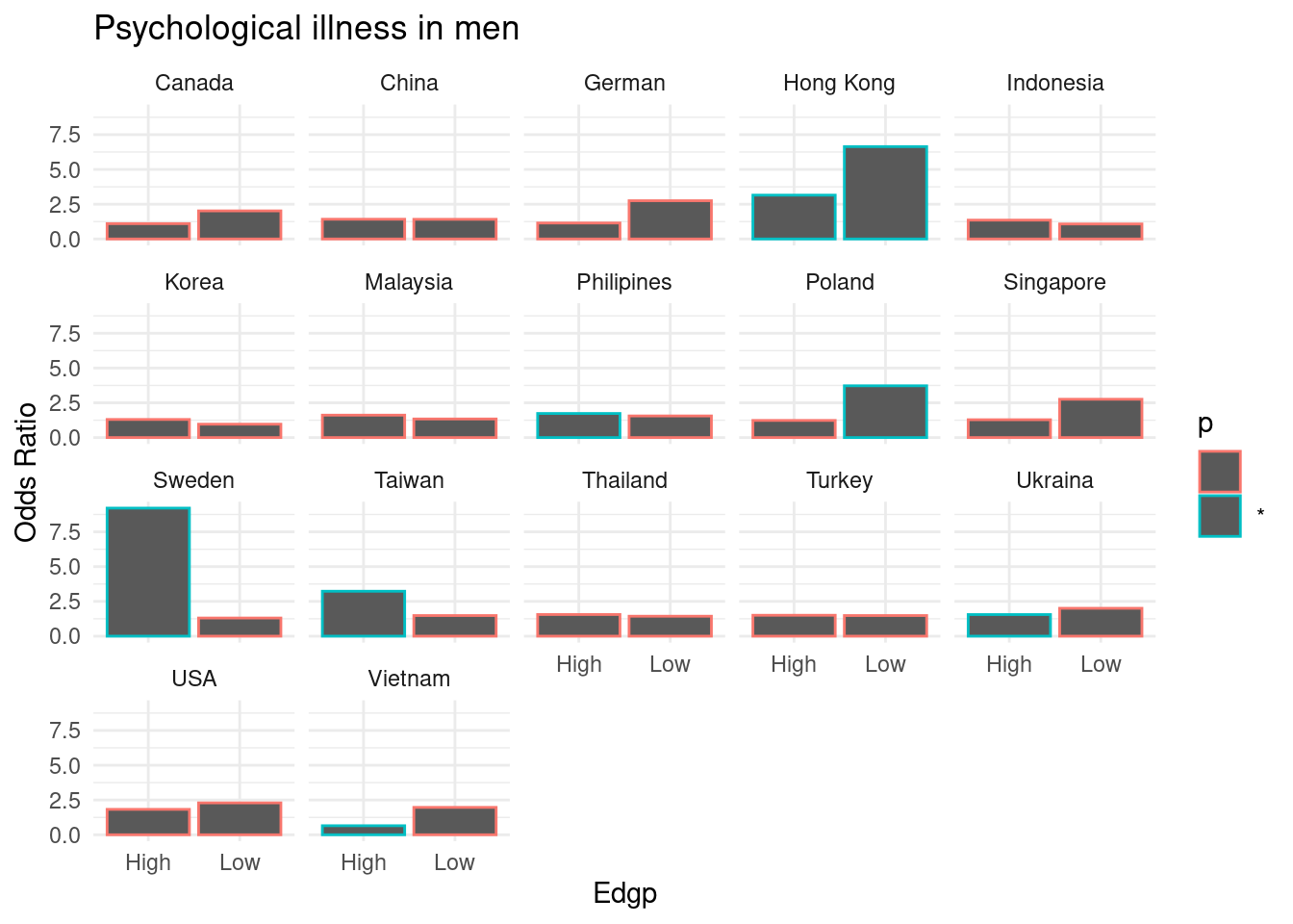
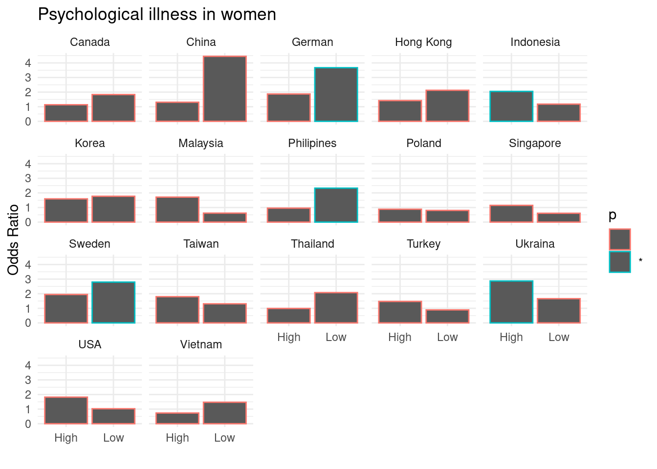
## as.factor(int2)4 0.08830323 0.10198420 0.865852 3.865713e-013.5.1 startication analysis by country
library(broom)
library(tidyverse)
mm5 %>% group_by(country_c, genders, Edgp) %>%
do(fit_country =
tidy(glm(family = binomial, data = .,
formula= TotalDepAnx ~ EcLoss + age))) %>%
unnest(fit_country) %>%
select(country_c:term, estimate, p.value ) %>%
filter(term == 'EcLossLoss') %>%
mutate(p = ifelse(p.value <0.05, "*", "")) -> repA
repA## # A tibble: 68 x 7
## country_c genders Edgp term estimate p.value p
## <chr> <chr> <chr> <chr> <dbl> <dbl> <chr>
## 1 Canada Men High EcLossLoss 0.0980 0.770 ""
## 2 Canada Men Low EcLossLoss 0.703 0.0640 ""
## 3 Canada Women High EcLossLoss 0.126 0.701 ""
## 4 Canada Women Low EcLossLoss 0.606 0.137 ""
## 5 China Men High EcLossLoss 0.350 0.253 ""
## 6 China Men Low EcLossLoss 0.346 0.665 ""
## 7 China Women High EcLossLoss 0.268 0.490 ""
## 8 China Women Low EcLossLoss 1.49 0.0744 ""
## 9 German Men High EcLossLoss 0.138 0.766 ""
## 10 German Men Low EcLossLoss 1.01 0.134 ""
## # … with 58 more rows