Chapter 9 TWAS

9.1 TWAS data prep

Now that we’ve completed a traditional GWAS analysis, lets run a Transcription Wide Association Study (TWAS). That is, testing the following hypothesis: Ho: No association between gene expression and trait. Ha: There is an association between gene expression and trait.

First we need to prepare the expression matrix. The expression data comes from the same 942 maize inbred lines used in the GWAS portion of the workshop (Mazaheri et al. 2019). Raw RNAseq reads were processed as described in (Zhou et al. 2020) to generate a transcripts per million (TPM) expression matrix for ~46,430 gene models in maize.

We will demonstrate how to create a subset of 501 genes sampled equally from the 10 maize chromosomes. The phenotypes used in this section are the same simulated phenotypes used from the GWAS section.

Packages used in this section are: (Dowle and Srinivasan 2021), tidyverse (Wickham 2021), rtracklayer (Lawrence, Carey, and Gentleman 2021), rrBLUP (Endelman 2019).

Load nececarry packages

library(data.table)
library(tidyverse)
library(rtracklayer)
library(scales)

Read in 942 expression matrix generated

setwd("~/PGRP_mapping_workshop/data/expression_data/")
expr = fread("widiv942_TPM.tsv", data.table = FALSE)

Keep only protein coding genes gff file

setwd("~/PGRP_mapping_workshop/data/gene_annotation_data/")
gtf <- rtracklayer::import('Zea_mays.B73_RefGen_v4.48.chr.gff3')
gtf_df=as.data.frame(gtf)
gff_gene = gtf_df[gtf_df$type=="gene",] # Protein coding genes

Keep needed columns from gff file

gff_keep_cols = c("seqnames","source","type","start","end","strand","gene_id","description","biotype")
out = gff_gene[,colnames(gff_gene)%in%gff_keep_cols]
genes_keep = out$gene_id
length(unique(genes_keep)) # 39,272 protein coding genes

Read in Metadata

setwd("~/PGRP_mapping_workshop/data/expression_data/")
name_convert = fread("01.meta_widiv942.txt", data.table = FALSE)
name_convert = name_convert[,c("SampleID","Genotype")]

Read in phenotypic data

setwd('~/PGRP_mapping_workshop/data/genotypic_and_phenotypic_data/')
phenos = fread("WIDIV_942.phe")

Add a row for gid to metadata

name_convert = rbind(c("gid","gid"),name_convert)

Gene coordinates of expression matrix

gene_loc = out[,c("gene_id","seqnames","start","end")]
colnames(gene_loc) = c("geneid","chr","s1","s2")

Keep only protein coding genes from .gff file

expr_sub = expr[expr$gid%in%gene_loc$geneid,]

Change sample names in columns to name in phenotyps file

names(expr_sub) = plyr::mapvalues(names(expr_sub), from = name_convert$SampleID, to = name_convert$Genotype)
colnames(expr_sub)[1] = "id"
rownames(expr_sub) = expr_sub$id

Check variance across all lines for expression in each data file

variance = data.frame(apply(expr_sub[,2:ncol(expr_sub)], 1, var))
variance$names = rownames(variance)
colnames(variance) = c("Var", "Gene")

Remove genes with zero variance

noVar = subset(variance, Var == 0)
noVar.genes = noVar$Gene
dim(expr_sub)
expr_sub = expr_sub[!expr_sub$id%in%noVar.genes,]
dim(expr_sub) # 38,593 genes

Remove genes not expressed in at least 5% of lines

low_expr = data.frame(apply(expr_sub[,2:ncol(expr_sub)], 1, function(x){sum(x == 0)}))
low_expr$names = rownames(low_expr)
colnames(low_expr) = c("Low_expr", "Gene")
Low = subset(low_expr, Low_expr > (ncol(expr_sub)-1)*0.95)
Low.genes = Low$Gene
expr_sub = expr_sub[!rownames(expr_sub)%in%Low.genes,]
dim(expr_sub) # 34,498 genes

Match name order to phenotype file file

phenos_order  = c("id",phenos$Taxa)
expr_sub = expr_sub[,order(match(colnames(expr_sub),phenos_order))]
identical(as.character(colnames(expr_sub)[2:ncol(expr_sub)]), as.character(phenos$Taxa))
gene_loc = gene_loc[gene_loc$geneid%in%expr_sub$id,]

Make quantile rank normalized gene expression matrix

mat = expr_sub[,2:ncol(expr_sub)]
dim(mat)
mat = t(apply(mat, 1, rank, ties.method = "average",na.last = "keep"))
mat = qnorm(mat /ncol(expr_sub))

Scale TMP values to be between -1 and 1 to be compatible with rrBLUP

mat = t(apply(mat, 1, rescale, to = c(-1,1)))
mat = cbind(expr_sub$id, mat)
colnames(mat)[1] = "id"

Make output file

mat_out = left_join(gene_loc,mat, by = c("geneid"="id"), copy = TRUE)

Keep only genes on chromosomes, remove mitochondrial and chrolorplast genes

chrm_keep = as.factor(seq(1,10,1))
mat_out = mat_out[mat_out$chr%in%chrm_keep,]
dim(mat_out) # 34,355 genes

Sample 50 gene models per chromsome and make sure to include P1

set.seed(123)
mat_sub = mat_out %>%
  group_by(chr) %>%
  sample_n(50)

See if P1 is in the filtered expression matrix

is_p1 = mat_sub[mat_sub$geneid=="Zm00001d028854",]
dim(is_p1) # Not in the subset data

Bind P1 expression to the matrix

p1 = mat_out[mat_out$geneid=="Zm00001d028854",]
mat_sub = bind_rows(p1,mat_sub)

Sort by chromosome and transcription start site from gff file

mat_sub = mat_sub %>%
  arrange(chr,s1)

Write the file

setwd("~/PGRP_mapping_workshop/data/expression_data/")
fwrite(mat_sub, file = "subset_widiv942_scaled_quant_rank_TPM.txt",col.names = TRUE, sep = "\t", quote = FALSE)

Look at histogram of expression of P1

hist(as.numeric(p1[,5:ncol(p1)]))

9.2 TWAS analysis

Load nececarry packages

library(data.table)
library(rrBLUP)
library(tidyverse)
library(rMVP)

Read in phenotypes

setwd("~/PGRP_mapping_workshop/data/genotypic_and_phenotypic_data/")
phenos = fread("WIDIV_942.phe", data.table = FALSE)

Read in expression data and put in the format for rrBLUP

setwd("~/PGRP_mapping_workshop/data/expression_data/")
expr = fread("subset_widiv942_scaled_quant_rank_TPM.txt", data.table = FALSE)
expr = expr[,-4]
colnames(expr)[1:3] = c("marker","chrom","pos")

Read A matrix

setwd("~/PGRP_mapping_workshop/data/genotypic_and_phenotypic_data/")
A.widiv = attach.big.matrix("WIDIV_942.kin.desc")
A.widiv = A.widiv[,]
mean(diag(A.widiv))  # = 2 because inbred lines

Check files are in the same order

identical(as.character(phenos$Taxa), as.character(colnames(expr[,4:ncol(expr)])))

Run rrBLUP for each trait and write out results

setwd("~/PGRP_mapping_workshop/twas_results/")
pheno_names = colnames(phenos)[2:3]

K only model

for(i in pheno_names){
  fitlist = list()
  fitlist[[i]] = GWAS(pheno = phenos[,c("Taxa",i)], geno = expr, K=A.widiv, min.MAF=0.0, n.core=10, P3D=TRUE, plot=TRUE)
  tmp = fitlist[[i]]
  colnames(tmp) = c("geneid","chrom","pos","p_value_log10")
  tmp$trait = i
  fwrite(tmp, file = paste("rrBLUP_TWAS_K",i,".txt",sep = ""),
         col.names = TRUE, sep = "\t", quote = FALSE, na = "NA")
  rm(fitlist)
}

K and SNP calculated PCs from K matrix in model

for(i in pheno_names){
  fitlist = list()
  fitlist[[i]] = GWAS(pheno = phenos[,c("Taxa",i)], geno = expr, n.PC = 3, K=A.widiv, min.MAF=0.0, n.core=10, P3D=TRUE, plot=TRUE)
  tmp = fitlist[[i]]
  colnames(tmp) = c("geneid","chrom","pos","p_value_log10")
  tmp$trait = i
  fwrite(tmp, file = paste("rrBLUP_TWAS_KandQ",i,".txt",sep = ""),
         col.names = TRUE, sep = "\t", quote = FALSE, na = "NA")
  rm(fitlist)
}

TWAS manhattan plot for Q and K model for high heritability trait

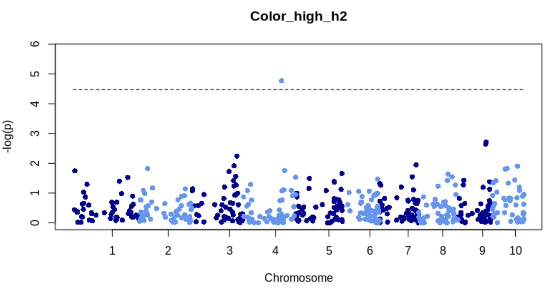
Read in results for Q and K model and make a scatterplot for most significant gene

k_q_model = fread("rrBLUP_TWAS_KandQColor_high_h2.txt")
sig_gene = top_n(k_q_model, 1, p_value_log10)
sig_gene_expr = expr[expr$marker==sig_gene$geneid,]
sig_gene_expr = data.frame(t(sig_gene_expr[,-c(2:3)]))
colnames(sig_gene_expr) = sig_gene_expr[1,1]
sig_gene_expr$Taxa = rownames(sig_gene_expr)
sig_gene_expr = sig_gene_expr[-1,]
plot_data = left_join(phenos, sig_gene_expr)
plot_data$Zm00001d052153 = as.numeric(plot_data$Zm00001d052153)

Plot it

sig_plot = ggplot(plot_data, aes(Zm00001d052153, Color_high_h2)) +
  # geom_jitter(colour = "darkorange",alpha = 0.3, width = 0.02) +
  # geom_boxplot(alpha = 0.5, fill = "plum3") + 
  geom_point(alpha = 0.5, fill = "plum3")+
  #ggtitle(paste0("BAF60.21 expression", " vs ", top_cis_snp)) +
  geom_smooth(method = 'lm',col="darkred", aes(group=1), se=TRUE)+
  theme_classic(base_size = 18)+
  ylab("Trait")+
  xlab("Scaled expression (TPM) Zm00001d052153") +
  theme(plot.title = element_text(hjust = 0.5))

setwd("~/PGRP_mapping_workshop/figures/twas/")
pdf("WIDIV_942_signif_TWAS.pdf", width = 6, height = 4)
sig_plot
dev.off()

Now do the same for P1

p1_gene_expr = expr[expr$marker=="Zm00001d028854",]
p1_gene_expr = data.frame(t(p1_gene_expr[,-c(2:3)]))
colnames(p1_gene_expr) = p1_gene_expr[1,1]
p1_gene_expr$Taxa = rownames(p1_gene_expr)
p1_gene_expr = p1_gene_expr[-1,]
plot_data1 = left_join(phenos, p1_gene_expr)
plot_data1$Zm00001d028854 = as.numeric(plot_data1$Zm00001d028854)

Plot it

p1_plot = ggplot(plot_data1, aes(Zm00001d028854, Color_high_h2)) +
  geom_point(alpha = 0.5, fill = "plum3")+
  geom_smooth(method = 'lm',col="darkred", aes(group=1), se=TRUE)+
  theme_classic(base_size = 18)+
  ylab("Trait")+
  xlab("Scaled expression (TPM) P1") +
  theme(plot.title = element_text(hjust = 0.5))

pdf("WIDIV_942_signif_TWAS_P1.pdf", width = 6, height = 4)
p1_plot
dev.off()

References

Dowle, Matt, and Arun Srinivasan. 2021. Data.table: Extension of ‘Data.frame‘. https://CRAN.R-project.org/package=data.table.

Endelman, Jeffrey. 2019. rrBLUP: Ridge Regression and Other Kernels for Genomic Selection. http://potatobreeding.cals.wisc.edu/software.

Lawrence, Michael, Vince Carey, and Robert Gentleman. 2021. Rtracklayer: R Interface to Genome Annotation Files and the UCSC Genome Browser.

Mazaheri, Mona, Marlies Heckwolf, Brieanne Vaillancourt, Joseph L. Gage, Brett Burdo, Sven Heckwolf, Kerrie Barry, et al. 2019. “Genome-Wide Association Analysis of Stalk Biomass and Anatomical Traits in Maize.” BMC Plant Biology 19 (1): 45. https://doi.org/10.1186/s12870-019-1653-x.

Wickham, Hadley. 2021. Tidyverse: Easily Install and Load the Tidyverse. https://CRAN.R-project.org/package=tidyverse.

Zhou, Peng, Zhi Li, Erika Magnusson, Fabio Gomez Cano, Peter A. Crisp, Jaclyn M. Noshay, Erich Grotewold, Candice N. Hirsch, Steven P. Briggs, and Nathan M. Springer. 2020. “Meta Gene Regulatory Networks in Maize Highlight Functionally Relevant Regulatory Interactions.” The Plant Cell 32 (5): 1377–96. https://doi.org/10.1105/tpc.20.00080.