Chapter 1 Contents

1.1 Histograms

Say you want to draw a histogram where the values are always positive (e.g. total revenue)

fortune <- read_csv("data/fortune1000-final.csv")

The default histogram binning behavior may be inappropriate. Use boundary = 0.5 to start the first bar at the minimum value, instead of centering it at the minimum value.¹ Here is the key part of the code.

default <- ggplot(fortune, aes(x = revenues, y = stat(density*width))) +
  geom_histogram(binwidth = 5000) +

adjusted <- ggplot(fortune, aes(x = revenues, y = stat(density*width))) +
  geom_histogram(binwidth = 5000,  boundary = 0.5) +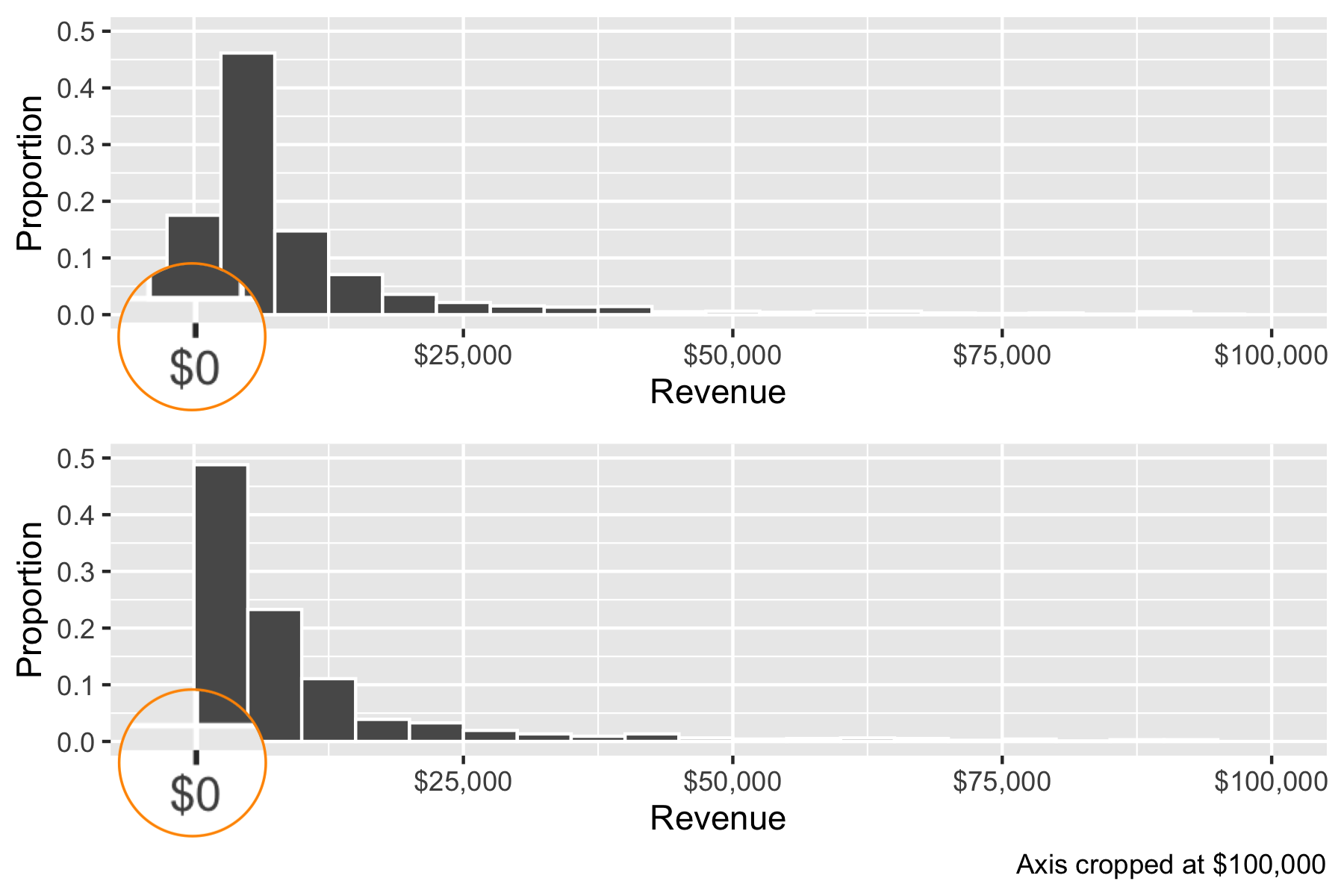

Notice that these two histograms are plotting the exact same data, and the widths of the bins are also the same. But because histograms require some user-defined way of binning continuous values, where the cutoff is set can change the what you see and the message.

1.2 The mean and sum of binary variables

Recall that TRUE and FALSE values are coerced to 1s and 0s. This leads to a very common “trick” to count the number of cases and count the proportion of cases that satisfy a condition.

data(gss_cat)

gss_cat %>% 
  group_by(year) %>% 
  summarize(
    p_notmarried = mean(marital != "Married"),
    n_notmarried = sum(marital != "Married"),
    n = n())

year	p_notmarried	n_notmarried	n
2000	0.55	1539	2817
2002	0.54	1496	2765
2004	0.47	1333	2812
2006	0.52	2340	4510
2008	0.52	1051	2023
2010	0.56	1153	2044
2012	0.54	1074	1974
2014	0.54	1380	2538

1.3 Packages

Do not keep packages that you do not use. This leads to errors like

library(Rmisc)

# Attaching package: ‘plyr’

# The following objects are masked from ‘package:dplyr’:

# arrange, count, desc, failwith, id, mutate, rename, summarise,
#     summarize

basically, what this message is saying is that the functions arrange, count, desc, failwith, id, mutate, rename, summarise, that were previously loaded by dplyr been replaced by other functions of the same name (in the plyr package)!!

1.4 Sampling

The Margin of Error for the sample proportion estimator \(\hat p\), at the \(\alpha = 0.05\) is

\[\mathit{MoE}_{\hat p} = 1.96\sqrt{\frac{p(1 - p)}{n}}\]

When we are in a hurry, a rough approximation to this number is to provide a ``conservative’’ estimate as \(\frac{1}{\sqrt{n}}\). Here is how this is an o.k. approximation:

\[\begin{align*} \mathit{MoE}_{\hat p} &\approx 1.96\sqrt{\frac{0.5(1 - 0.5)}{n}} \because \text{the most conservative estimate for } p\\ &= 1.96 \frac{\sqrt{0.5\times 0.5}}{\sqrt{n}}\\ &\approx 2 \frac{\sqrt{0.5\times 0.5}}{\sqrt{n}}\\ &= \frac{2 \times 0.5}{\sqrt{n}}\\ &= \frac{1}{\sqrt{n}}\\ \end{align*}\]

The numerator of the standard error is a second-order polynomial that reaches its maximum at \(p = 0.5\). In other words, \(\arg \max_p p( 1- p ) = 0.5\). To see this, draw \(p( 1- p )\) as a parabola \(-(p - 0.5)^2 + 0.25\). Larger standard errors are more conservative (they reduce the chance that you get a \(t\)-stat of more than 2), so this value that makes the numerator at its largest value is a conservative estimate.

Thanks to Maria Mercedes for pointing this out.↩