12 Appendix A - Installing R and RStudio and writing a script
Abstract
This chapter introduces the open source statistical computing software program called R, and the accompanying interface software called RStudio. The goal is to walk a user through the installation process, review some of the basic features of the software, and write a first script.
Keywords: Script, dataframe, commands, syntax
12.1 R and RStudio
The chapter introduces you to R and RStudio, statistical computing soft- ware that is commonly used in econometrics. R is an open source programming language and software environment for statistical computing and graphics. It is widely used by statisticians and other “number crunchers” for data analysis and related applications. R provides most of the data management and econometric tools needed to manipulate and analyze data. Being open-source, the R development community provides free add-in “packages” that expand and enhance R’s capabilities. A separate appendix introduces you to R Markdown, which is a way of using R to create reports that integrate statistical analysis results (visualizations of data, tables of statistical analysis) with text commentary.
R is most powerful as a “scripting language.” A script is a text file that contains a sequence of commands that you submit to R. You submit commands for processing by highlighting a command, or by highlighting a set of commands, and clicking the “run” button. R then executes, in sequence, the commands you have highlighted, much as a cook might follow the steps of a recipe. Like baking with a recipe, running command through a script has an important constraint. Once you have run a command you often cannot “undo” it. Once you have mixed eggs in with the flour, when baking from a recipe, you cannot separate them. Unlike baking, in data analysis you can always start over at the beginning with practically no cost or effort, and simply re-run commands from the beginning of the script.
Scripting is very important because it provides an easy way to fix mistakes, to insert or delete commands, to repeat what one has programmed without having to re-enter everything, and to give others an opportunity to replicate work.
In this chapter, we will offer guidance to help you install R and RStudio on your laptop or desktop computer, and write a first script. We will execute, or run, some preliminary commands to install supplemental packages, read in some spreadsheet data, and run some simple commands to generate summary statistics.
Statistical analysis involves manipulating data, so the most important first thing to learn is how to get data into the R programming environment. R stores data in a format that R users call a dataframe. For most purposes, this is equivalent to a dataset, or spreadsheet, but R can also associate single numbers (scalars), lists and other vectors, and labels, etc. with a dataset. A dataframe is broader than just a dataset.
Our approach emphasizes the usage of scripts. Good data analysis practice is to start with a raw, original dataset or spreadsheet and then have every single manipulation or transformation of or calculation with the original dataset recorded in a script. That way, any person can take the original data and replicate the analysis. Perhaps they (or you) will find a mistake.
A script is vastly superior to a software program like Excel that is used to analyze data in a spreadsheet form. If you use Excel to transform data (by, for example, creating a new variable based on existing data) there is often no record of the transformation (except in your head). Most social scientists transformed their data extensively in Excel prior to statistical analysis. They are no longer able to reproduce those transformations. Many studies from before the year 2000 are not replicable. The authors of the studies have no records, and have likely forgotten, how they transformed the data. It was not common practice in the social sciences, until the early 2000s, to insist on a script enabling replication.
Writing a script mostly involves cutting and pasting commands that R will recognize. The commands have to follow the proper syntax. The word syntax here means the arrangement, of words, character, and punctuation marks in an order that R can understand. Just as the sentence, Men a three boat in are sinking that is. is not proper English grammar syntax, so too will some commands in R be in proper syntax and others will be in improper syntax. Moreover, the order or sequence of commands themselves can be a proper order or an improper order. Learning what is proper syntax is what software engineers and coders do. This book is not about coding: we will be happy to cut and paste well-written code, and simply change variable names and options. But you will need to know some syntax, just like the learner of any language needs to learn syntax.
We will use the interface called RStudio to edit and run R scripts. RStudio and R have to both be installed on your computer. Once they are installed, you only need to start RStudio, as it will automatically open R for use. RStudio is an interface, or a shell, in which R is embedded.
Any standard Mac or Windows personal computer will work fine for run- ning R. Computers with Linux as operating system may also be used, but installation may be a bit more complex. You can often buy a new laptop for less than $400, and an adequate used laptop for less than the cost of a textbook. Some tablet computers (such as the Surface) may be compatible with RStudio. The Ipad cannot be used with RStudio at the time of this writing. RStudio has an online version that you may use for free with a guest account (you can search the web for the words “Posit cloud” or go to https://posit.cloud/). You may also find R and RStudio installed on library lab computers.
We recommend that you also purchase an inexpensive external mouse for your laptop. You will do a lot of highlighting of sections of code, which is much easier with a mouse than with a finger and touchpad. Investing a few dollars in a mouse will repay itself many times over in saved frustration.
For most people, the goal in using R for data analysis to analyze data, not to write complex computer programs. The typical R user spends time copying, pasting, and modifying scripts that have already been written. Therefore, throughout the book we provide you with sample scripts that you can modify rather than write from scratch.
12.2 Installing R and RStudio
To get started, you need to download and install two different free soft- ware packages: R and RStudio IDE. R is maintained by CRAN, the Comprehensive R Archive Network. CRAN is a collection of sites that carry identical material, including downloads of R, extensions, documentation, and other R related files. R is available for many platforms, and below are download instructions for Mac and Windows. RStudio IDE is maintained by Posit, an independent public benefit corporation that has pledged to maintain RStudio as open-source software.
You should install R first before Rstudio. So do the following first! Download and install the software program for R. Visit the CRAN website: https://cran.r-project.org/. Click on the download link corresponding to the operating system that you will be using to run R. For most people, that is Mac or Windows. You may at some point be asked to choose a CRAN mirror server from a long list. A mirror is a server that maintains everything R related. It does not matter which one you pick. Follow the instructions, depending on your operating system.
MAC users need to determine which version of the Mac operating system (OS) they are running, and click on the appropriate version of R. You can find your OS version by clicking on the Apple icon in the upper left and then “About This Mac.” After the install package has been downloaded, find it (probably in your Downloads folder) and double click. Installation may be automatic, or you may have to follow some instructions to properly install the program.
Windows users need to click the link that says “install R for the first time.” After downloading the install package, which probably can be found in your Downloads folder (it will be a file ending with .exe), double click on the file to run the .exe file, and follow the installer’s instructions. Typically nothing needs to be done other than clicking either “next” or “I Agree” every time, accepting the default settings.
Once you have installed R, you could access and run it by clicking on the icon that might now be on your desktop or among your programs. However, as mentioned above, we will be interacting with R through the RStudio interface.
To install RStudio go to the RStudio website at https://posit.co/. In the “Products” menu you will find a link to the RStudio IDE. Follow the instructions to download and install. You will want to free open source edition. On Windows machines, after the download, go into your Downloads folder and double click on the downloaded package to install.
If you have an older Mac (running an older operating system), you may need to install a different version of RStudio. Seek help! Better yet, just buy a cheap Windows laptop. ;-)
A typical problem when installing is that someone else set up your computer and you do not have “administrator” privileges when you use the computer. If that is the case, logout and re-boot your computer by logging in as the administrator, and then install R and RStudio. Another typical problem for Mac users is that you open and run RStudio from your download folder instead of doing a proper installation. When users do this, they end up “in- stalling” RStudio repeatedly. So be careful. More the RStudio application to your applications folder. Ask for help if you have little experience installing a program on your computer.
12.3 Getting to know your way around RStudio
Open the RStudio program. When you start RStudio for the first time, the screen will look something like the screenshot on this page. The left frame is the R Console. This is where commands could be entered one by one, if you wanted to run R interactively. We will not usually enter commands this way—instead, we will use the script editor. When you open RStudio it automatically opens R. You do not have to open R separately.
Let us open the script editor and start a simple R script. At the top of the window, use the drop-down menus to select File → New → R Script. You should see something like the screenshot above. The top left frame that is now opened up is an area where you write and edit scripts: the R Script Editor. A script is simply a set of executable commands that can be run in chunks or all at once.
The screen shot shows the four basic windows or boxes you will be using once you get up and running in RStudio. You can change the size of the different frames by hovering on the line between two frames and then clicking and dragging. The Script Editor (upper left) is where you will view and edit your R scripts (commands). Notice that in the lower left corner of the window is a toggle dropdown menu: you might find yourself using this to switch between R script mode and R Markdown mode. The Console (lower left) is where R is actually running, and where most of your data analysis results will appear. The Workspace or Environment (upper right) shows data sets and variables you have loaded or created. Usually you want to be in the Environment tab. The Session Management window (lower right) has tabs for various R-related files, plots (graphics) you have created, packages (program add-ins to do a variety of tasks), and help.
Type (or cut-and-paste) the following line of script into the script editor (it works like a simple word processor):
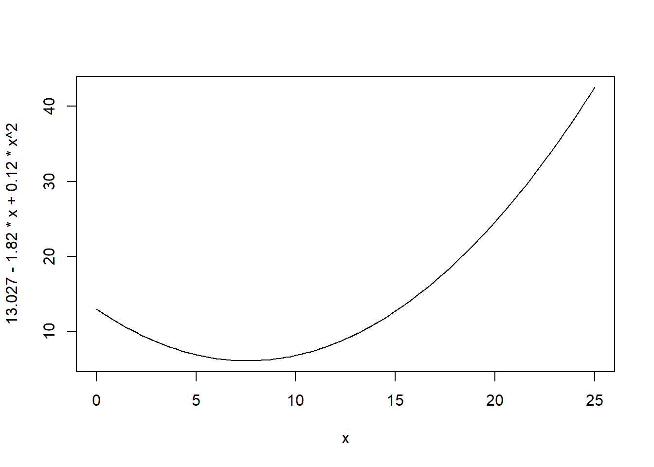
Notice that when you type or paste the line of script nothing happens. The script has to be “run.” Before we do that, take a look at the syntax of the command in the script. The curve() command is a command in “base R” (many commands we will use in this book are in supplemental packages). As the name suggests, the command will draw a curve. Inside the parentheses of the command are two terms, separated by a comma. The first term is a polynomial, more precisely a quadratic equation (one of the x terms is squared), that gives the values for y for different values of x. The range for the x-axis is given by the second term (many of the terms inside commands are called “options”). This term is xlim=c(0, 25). It defines the limits of the x-axis to be between 0 and 25. The expression c() is standard base R syntax to define a vector, an ordered set of numbers or other elements. In the case the vector has two elements, the lower limit 0 and the upper limit 25.
Highlight the line in the script containing the curve command, or put your cursor in the line, and press the run button with your cursor. You should see a curve appear in the plot window on the lower right. (You may have to click on the “plots” tab.) Type in a different equation on the following line (you may cut and paste the existing line, and then modify, rather than retyping everything) and see what happens.
In many contexts, you will be obtaining data from some external source, often as a spreadsheet. Let us import data on education attainment and earnings for a sample of people in Kenya. The data was collected by the government of Kenya as part of a regular nationally-representative survey of households in the country.
# Read Kenya earnings data from a website
url <- "https://github.com/mkevane/econ42/raw/main/kenya_earnings.csv"
kenya <- read.csv(url)
The important command in this line of code is the read.csv() command on the second line; it reads into R a spreadsheet. Most data that you will analyze will come in the form of a spreadsheet, which organizes data in rows and columns. The Excel format (with file extension .xls or .xlsx) is the most common format for spreadsheets. But a simpler format, called the “comma separated value” or csv format, can be loaded into R with ease. Any Excel file that you have can be saved in .csv format, but be careful because a .csv file can only be one worksheet of an Excel file and it will not have formulas or formatting. Inside the read.csv() is a website address (a url) for the csv file. In the code, we first assign the web address (the Uniform Resource Locator, or url) and then use the command kenya <- read.csv(url) to read the data addressed by the url, and assign it to the object kenya in the environment. Notice the use of “<-.” This is called the “assignment operator.” You are assigning a label to an object in R. It is almost always equivalent to “=.” We use a mix of “=” and <- in this book, since social scientists commonly use both. In this case, the spreadsheet, when read into R, will be called kenya.
Run the two lines of code. Look under Data in the Environment pane (upper right). You should now see the object kenya in the environment, with 15 variables. If you click on the blue expando button next to the kenya in the environment window, this will display the variable names and a small preview of the data. You will also see, in the Environment, the object url, which is the website address.
Click on the dataframe name, kenya. This should open the dataset in what looks like a spreadsheet in the script editor window. Take some time to examine the spreadsheet.
The units of observation (individuals) are in the rows, and variables are in the columns. Most of the values taken by variables are integers or numeric, in the sense that each individual value is a number, but one variable wealth_group contain words or letters, such as “poorest”. This kind of variable is called a string variable or a character variable. When R reads in a spreadsheet file, it takes its best guess as to what kind of variable it is, string or numeric. If R detect a string variable that only has a limited number of character patterns, it might decide to import the variable as a factor variable. A factor variable is categorical, and qualitative (not quantitative): thus an observation (individual) is either rich or poor or middle. A factor variable is actually a vector of integer values with a corresponding set of character values, called the levels, which are used whenever the factor variable is dis- played. Another kind of variable is a logical variable that takes on values TRUE or FALSE, and R knows to use 1 and 0 for these as appropriate.
We can see all the variables in the kenya dataframe with the names() command.
names(kenya)## [1] "educ_yrs" "age" "month_interview"
## [4] "wealth_group" "female" "rural"
## [7] "earnings_usd" "years_lived_elsewhere" "christian_main"
## [10] "christian_evang" "muslim" "kikuyu"When we refer to a variable in R code, the format is the name of the dataframe (kenya), then the $ sign, followed by the variable name (wealth_group), all with no spaces. Hence kenya$wealth_group is the variable wealth group in the dataframe kenya. This way R knows which dataset to look in, if you have more than one dataset in the environment. Some commands allow you to specify the dataframe just once, rather than repeating it for every variable. These commands, written to be part of what is known as the “tidyverse,” employ a coding technique called piping that obviates the need to continually restate the dataframe. In a piped command, the dataframe is piped through a series of commands that understand they are manipulating variables in the dataframe.
Now let us create a new variable in our dataset. In the dataframe we have variables for the number of years lived elsewhere (not in the village or town where the survey was conducted) and the person’s age. So we can create the ratio or years lived elsewhere to age; this would be the proportion of a person’s live lived elsewhere, and should be between 0 and 1 if the variables are measured correctly. Highlight and run the next line:
kenya$prop_life_elsewhere = (kenya$age/kenya$years_lived_elsewhere)This creates a new variable in the dataset, prop life elsewhere. Look in the environment at the kenya dataframe (use the blue expando button) to see that the new variable is there.
We can also create new variables that are logical variables, and convert them into numeric binary variables.
kenya$low_earner = (kenya$earnings_usd<200)This creates a new variable in the dataset called low earner, which takes the value TRUE if the earnings (earnings usd) are less than 200 dollars, and FALSE otherwise. This variable is a logical variable. Click on kenya again and look at the data. The very last variable is the new variable low earner. Note that it takes values of “TRUE” or “FALSE”. In many applications, R treats TRUE as the number 1, and FALSE as the number 0. We can explicitly convert the variable into a numeric variable that takes on value 0 or 1 with the following command:
kenya$low_earner = as.numeric(kenya$low_earner)We call such a variable a binary or dummy variable. You can also create new variables using mathematical formulas, such as
kenya$earnings_usd_sq = kenya$earnings_usd^2This creates the square of earnings. Notice how we add the suffix sq to make the new variable name different from the original variable and at the same time indicate it is the square. Math expressions in R are generally similar to Excel. We can also use the commands of the tidyverse package to create new variables. Consider:
library(tidyverse)
# create new variable using tidyverse pipe syntax
  kenya <- kenya %>% mutate(earnings_usd_cu = earnings_usd^3)
The syntax here is called “piping” or sometimes the “tidyverse” syntax. Imagine a pipe. Data flows into the pipe. We can think of the dataframe as an object. The data object is transformed by R. Then a new object continues to flow through another pipe, where it may be transformed or changed again. After every pipe segment, a data object emerges. The final data object may be stored in the environment, provided it is named. In an odd quirk of piping, the general syntax in common usage is to start with the assigning of the name of the final object, using the assignment operator. So the syntax of this command is as follows. We start with the name of the new dataframe to be used to store the results of the pipe, once the old dataframe is changed. In this case, we assign the new dataframe to the same name as the old dataframe, so it replaces kenya. Then we start the pipe, first by “getting” or “calling” the dataframe kenya. We pipe kenya, using the pipe operator %>%, into a command called mutate to create the new variable. The new variable is the earnings variable raised to the power 3. We add the suffix cu to create the name of the new variable.
The advantage of the pipe syntax is that we do not have to put the
dataframe name and the dollar sign $ before every variable name. R “re- members” that the variables are in the dataframe. The shortcut for the pipe operator %>% is Cmd-Shift-m on Apple Mac computers and Ctrl-Shift-m on Windows computers.
Factor or categorical variables can be created from numeric variables. For example, the cut command will create a new variable that takes on three levels according to the earnings variable. We can create the new variable in two ways. First, using the $ address syntax. Second, using the piping and mutate syntax.
kenya$earnings_group = cut(kenya$earnings_usd, 3)
kenya <- kenya %>% mutate( earnings_group=cut(kenya$earnings_usd, 3))
Another way to create new variables is to use logical conditions such as ifelse. Consider for example the following command:
# create a new variable using basic tidyverse syntax
  kenya <- kenya %>% mutate(
    what_level_educ =
    ifelse(educ_yrs>=10 , "high",
    ifelse(educ_yrs>4, "medium",
    ifelse(educ_yrs>0, "low",
    "none or missing"))))
The command creates a new variable that takes on four values according to the value of the education variable. The first condition says the new variable indicating the education level should be the word high if the person has more than 10 years of education. If that is not the case (the “else”) then the level should be medium if education is greater than 4. If that is not the case (else again, so if education is neither higher than 10 nor higher than 4), and if education is higher than 0, the level should be low. Finally if none of the conditions are met, the level should be “none or missing.” Notice how many parentheses are needed to balance the opening parentheses. A major problem in R syntax for novice users is ensuring that all parentheses are balanced.
You can run the script a couple of different ways. Often, we will want to run just a part of the script. To do this, highlight the section of your script you want to run and press the run button located at the top right of your Script Editor. Sometimes it is more convenient to click on the line number, which will then highlight the line itself. You can also click and hold to highlight a set of lines by moving over the line numbers. Note: Here is where you will start to see the advantages of using an external mouse and not your touchpad! If you are just running one line, then you do not need to highlight the line. Instead, put your cursor anywhere in the line, and then click the run button.
Instead of clicking on the run button, many users find it easier to run commands from the keyboard. On a Windows machine, Ctrl+Enter will run commands. On a Mac +Enter. The Enter key is sometimes labeled as the Return key.
Another useful shortcut on Windows is Ctrl+Alt+B, and on the Mac +Option+B, which runs all the commands from the beginning of the script to the current line where the cursor is located.
Alternatively, if you want to run the whole script, you can go to the Code tab at the top and click on Run Region, then select Run All.
Once you run the script, you should notice a couple of things. First, you should see the output of the script (as well as the code that was run) in the R Console, which is the frame in the lower left directly underneath your script editor. Second, you should also notice that the top right box, which is your Workspace or Environment, is no longer blank. Your Workspace shows you everything (in R language they are called “objects”) that you have created during your current or most recent session using R. These objects may include dataframes, values, vectors, functions, and other objects. Entire workspaces can be saved and reopened later. We encourage you, though, to never save the workspace (always click “no” when prompted when you close RStudio, and instead save your script.)
The bottom right box, the Session Management area, is where you can access your files (saved scripts, plots, etc.). You can also access your installed packages (more on packages later), and you can get additional help if need be. Plots will appear here as well. We prefer not to use interactive menus in this area.
12.4 Packages
A package in R is like an “add-in” for Excel or a downloadable app for your phone. Some statistical commands come as standard equipment with R, but many commands are coded in packages and must be downloaded and installed. A package has its own set of commands and help documentation. You can type any package name and R into Google, and you will almost always find helpful hints, summaries and documentation.
Among the many packages we will use in these tutorials are sandwich, tidyverse, WDI, modelsummary, and haven. We will see what they do later. Packages need only be installed once onto your computer. This process down- loads some files and makes them available to R. If you change computers, or update your operating system, or install a newer version of R, the packages will need to be installed again. Type and run the following commands:
``` r
#install.packages(c("modelsummary", "tidyverse", "sandwich"))
#install.packages(c("WDI", "haven", "readxl", "estimatr"))
```
Notice that c() has in the parentheses a list of packages, each separated by a comma. Notice the double parentheses at the end of the line. That balances, or closes, the open parentheses. An alternative, install.packages("tidyverse")
will install just one package. The command can be copied and the name of the package replaced, to install another package.
Check that you are connected to the Internet, and then highlight the com- mands in the script and click on “run” to install the packages. You should see in the Console (lower left) that the packages are being installed. You will see a lot of red comments and text appearing. This does not necessarily in- dicate a problem. R uses red script sometimes simply to highlight important information. So skim the script that appears; unless it explicitly says that the install failed, you are fine.
Sometimes when you install a package, you will see a comment appear that you should install some other package. usually, you can just click yes. Sometimes, though, for Mac users, R asks whether you want to install a binary version of a package and have your computer compile the binary version. In our experience, it is better to respond with “no.” You respond by clicking on the blank space at the end of the question, after the yes or no options, and type the letter “n” and then hit the Enter key.
Sometimes installing a package does not work. For example, you might receive the following message when installing an R-package (on a Windows computer):
‘lib = "C:/Program Files/R/R-4.2.2/library"’ is not writable
Close RStudio. When prompted to save the workspace, click no. That is, do not save the workspace. It is generally good practice to open R Studio with a clean slate.
12.5 Create a folder for your scripts and data
It is desirable to have your saved scripts and data in a working directory, a folder in your computer. You should create this new folder in whatever folder you use for course work, preferably not in the cloud, but on your computer’s hard drive. For example, a folder name might be Classes/econ42. Once you create the folder, you will need to know its full “path” name. For example, in Windows the path might be: C:/Users/mkevane/Documents/Classes/econ42
while on a on a Mac it might be: /Users/mkevane/Documents/Classes/econ42.
Of course, unless you are Michael Kevane (or Micah Kevane), your user- name will be different. You can find the full path using Finder on a Mac or Explorer in Windows. Note that the Mac uses forward slashes and Windows uses backwards slashes. In a programming quirk, R only recognizes forward slashes, so that in your R code, the working directory for a Windows machine will be written as, for example:
C:/Users/mkevane/Documents/Classes/econ42
12.6 A first script to save for later reuse
Start RStudio again. Remember that this also opens R; you do not need to open R separately. Click on the File option in the menu in the upper left, select New File, and then select R script. The script window will open, ready for you to start typing in a blank script. As noted above, a script is just a file that contains a set of instructions for R to implement, along with comments for the user that explain (to future users) what the commands are doing.
Recall that lines with hashtag symbol # at the beginning will be ignored by R. We use these lines to write comments and other information about what the script is doing, and to break the script into sections. It is good practice always to follow a standard format for your R scripts, with a brief title, then your name and the date, followed by a short description of what the script does. This is useful information for your future self (a year from now you might want to use a script, but without the comments you may no longer remember what the script is doing). Every line that is part of a comment must start with a # sign, or else R will treat it as a command and give you an error message when you try to run it.
Here is what you should have at the top of the script. You may type this, or cut and paste, and change to have your name and the current date.
#=======================================================
# Description: Kenya earnings data preliminary analysis
# original Natalia Lafourcade 7/1/2025
# Latest version: Oscar Hijuelos 9/1/2025
#=======================================================
Following the title and description, the script is organized into three main sections: • Settings, load packages, and options • Data section • Analysis section
The Settings section loads packages and locations of datasets that you might use or import for analysis. In the data section, you will import your dataset, create any new variables, and create any sub-samples of the data. In the analysis section, you typically first run some descriptive statistics to see what is in the data. Then you add commands that will create tables and plots to describe the data, and conduct any analysis. In particular, you will have R carry out regression analysis. A command in R is a word that instructs R to carry out some calculations or some operation, with some objects that are in the environment.
6.1. The Settings section of the script
The first main section of the script should be demarcated with the fol- lowing header, which you may type or cut and paste.
#==========================================
# Settings, load packages, and options
#==========================================
The code in this section sets your working directory, loads the packages we will often use in this course, turns off scientific notation so numbers will be easier to read, and does a few other useful things. This section or one very similar should be at the start of each of your scripts.
The first command in every script is an instruction to R that will clear your working space, which means it will remove datasets and results that are in R’s memory. This is like starting your R session with a clean slate.
Notice the command starts with rm which stands for remove, and the second part in the parentheses instructs R to remove everything that is in the list=ls() which by default is everything in the environment.
Once you have cleared the environment, you need to set the working directory so that when you ask R to import and save datasets and results, R knows where to find them or where they should go on your computer. To set the working directory it is useful to use the menus at the top in RStudio. Go to the Session tab or option. The dropdown menu will have an option “Set Working Directory” and you should choose that. That leads to the dropdown choice “Choose Directory…” and you should choose that. Now navigate through your folders to find the folder you created for the class, and click on “Open.” In the Console window (lower left) you will see the setwd() command, and inside the parentheses will be the file path to your folder. Copy the line of code in the Console (starting with the setwd) and paste into your script. Reminder: whether you use a Mac or Windows machine, the slash symbols in the setwd(...) path must be forward slashes, not backward slashes.
``` r
# Set working directory
# (edit for YOUR folder)
# setwd("/Users/mynamehere/econ42")
```
In general, when setting your working directory, it is best not to only use the menu system. Instead, always copy the setwd() from the Console, or from a previous script, and paste the command in your current active script. That way, your future self, and others, will always be able to replicate your work.
Whereas you only have to install a package onto your computer once, packages you want to use for analysis must be loaded into R every time you start a new R session. See the earlier discussion about installing packages. The library() command loads the packages. By including these commands in all your scripts and running them every time you start up RStudio, you will not need to worry about remembering to do it.
# Load the packages
# (must have been installed)
 library(tidyverse)
 library(modelsummary)
 library(haven)
 library(sandwich)
 library(estimatr)
The remaining lines of code in the settings section set the rule for usage of scientific notation for numbers (90000000, and not 9E7) and limits the number of decimals in some displays of tables (3.458 and not 3.45834529034).
Now run the entire Settings section of code as a block if you have not run it already. Highlight all the lines from the very top of the script through all of Section 1 (remember you can also highlight by clicking on the line numbers rather than the actual lines), and click the Run button. You should see in the Console (lower left) that the packages installed are being loaded. You will see some text appearing. This does not necessarily indicate a problem. R uses red script sometimes simply to highlight important information. So skim the text that appears in the console; unless it explicitly says that the package is not found, you are all right. Once your packages are loaded, click on the Packages tab in the Session Management box (lower right). You should see the names of the packages you added in the list, with check marks for the ones that are loaded.
6.2. The Data section of the script
The second section of the script should be demarcated with the following header, which you may type, or cut and paste.
#==========================================
# Data
#==========================================
The data section of a script typically contains commands that read in (or load) data. In this book we will occasionally create simulated data. This means that we will have a few commands that create a dataframe. They will be reviewed later.
Here, we will once again read in the Kenya earnings dataset, and create a new variable.
# Read Kenya earnings data from a website
    url <- "https://github.com/mkevane/econ42/raw/main/kenya_earnings.csv"
    kenya <- read.csv(url)
# Create a new variable
kenya$prop_life_elsewhere = (kenya$age/kenya$years_lived_elsewhere)
6.3. The Data analysis section of the script
The third section of the script should be demarcated with the following header, which you may type, or cut and paste.
#==========================================
# Data analysis
#==========================================
Now that data has been loaded into R, it is time to analyze it. Analysis generally takes three forms: tables of descriptive statistics and comparative statistics, graphical displays called figures (also known as charts or plots), and regression analysis.
A table of descriptive statistics usually includes the mean, standard devia- tion, median, etc. We can create such a table using the command datasummary in modelsummary, one of the packages that we loaded. Run the following line of code:
datasummary(All(subset(kenya, earnings_usd<=1000)) ~ Mean + SD + Median + (N=length),
data=subset(kenya, earnings_usd<=1000),
title="Kenya earnings dataset")| Mean | SD | Median | N | |
|---|---|---|---|---|
| educ_yrs | 9.54 | 3.95 | 10.00 | 20829.00 |
| age | 32.78 | 9.16 | 32.00 | 20829.00 |
| month_interview | 4.24 | 1.38 | 4.00 | 20829.00 |
| wealth_group | 3.19 | 1.35 | 3.00 | 20829.00 |
| female | 0.57 | 0.50 | 1.00 | 20829.00 |
| rural | 0.57 | 0.50 | 1.00 | 20829.00 |
| earnings_usd | 220.17 | 213.26 | 139.53 | 20829.00 |
| years_lived_elsewhere | 28.07 | 10.38 | 27.00 | 20829.00 |
| christian_main | 0.57 | 0.50 | 1.00 | 20829.00 |
| christian_evang | 0.29 | 0.46 | 0.00 | 20829.00 |
| muslim | 0.08 | 0.27 | 0.00 | 20829.00 |
| kikuyu | 0.17 | 0.38 | 0.00 | 20829.00 |
| prop_life_elsewhere | 1.00 | 20829.00 |
We can obtain descriptive statistics separately for selected variables. You can do this by running the following command in the script (try it).
datasummary(age + earnings_usd + educ_yrs~ Mean + SD + Median + (N=length),
data=subset(kenya, earnings_usd<=1000),
title="Kenya earnings dataset")| Mean | SD | Median | N | |
|---|---|---|---|---|
| age | 32.78 | 9.16 | 32.00 | 20829.00 |
| earnings_usd | 220.17 | 213.26 | 139.53 | 20829.00 |
| educ_yrs | 9.54 | 3.95 | 10.00 | 20829.00 |
We can also select a subsample of the dataframe. Often we will want to run our analysis on a subset of the observations that have some specific characteristic(s). The easiest way to do this in R is using the subset(...) function. Examine and then run the next line of code:
datasummary(age + earnings_usd + educ_yrs ~Mean + SD + Median+(N=length),
subset(kenya, female==1 & earnings_usd<=1000), title="Kenya earnings dataset, women only")| Mean | SD | Median | N | |
|---|---|---|---|---|
| age | 32.71 | 8.44 | 32.00 | 11818.00 |
| earnings_usd | 183.15 | 197.22 | 116.28 | 11818.00 |
| educ_yrs | 9.60 | 4.03 | 10.00 | 11818.00 |
The code replaces the name of the dataset (kenya) with the following: subset(kenya, female==1 earnings usd<=1000). This uses only the ob- servations that have the property female equal to 1 and earnings less than or equal to $1,000. The double == sign is used to indicate that you want only the observations where the condition is exactly true. Use the symbols “&” for “and” and the “|” for “or” for more complex subsetting, such as:
  kenya_new = subset(kenya, female==1 & earnings_usd<=1000 &
    educ_yrs<20)
Based on this command, can you tell which individuals will be included in the new sample? If you were to run a command like this, note that here a new dataframe called kenya new is created; you would see it in the Workspace environment window with fewer observations than the original dataframe kenya.
The table command will provide a count of the number of observations in each category of a categorical variable, such as county. Run the table commands and see what happens.
# frequency tables by wealth group
table(kenya$wealth_group)
##
## 1 2 3 4 5
## 3218 3671 4390 5699 5108
table(kenya$wealth_group, kenya$female)##
## 0 1
## 1 1595 1623
## 2 1813 1858
## 3 2097 2293
## 4 2462 3237
## 5 1758 3350Notice that in the earlier commands, we restricted the observations to be those with earnings less than or equal to $1,000. In the table command, we do not have this restriction. We can restrict or subset the sample in base R, but it is a bit clunky. We use the square brackets after the dataframe name [], like this:
# frequency tables by wealth group
table (kenya$wealth_group[kenya$earnings_usd<=1000])
##
## 1 2 3 4 5
## 3198 3634 4299 5467 4231
table(kenya$female[kenya$earnings_usd<=1000],
kenya$wealth_group[kenya$earnings_usd<=1000])
##
## 1 2 3 4 5
## 0 1581 1781 2026 2317 1306
## 1 1617 1853 2273 3150 2925The tidyverse syntax is simpler:
# frequency tables by wealth group
  kenya %>% filter(earnings_usd<=1000) %>%
    group_by(wealth_group) %>% tally()
## # A tibble: 5 × 2
## wealth_group n
## <int> <int>
## 1 1 3198
## 2 2 3634
## 3 3 4299
## 4 4 5467
## 5 5 4231## # A tibble: 10 × 3
## # Groups: wealth_group [5]
## wealth_group female n
## <int> <int> <int>
## 1 1 0 1581
## 2 1 1 1617
## 3 2 0 1781
## 4 2 1 1853
## 5 3 0 2026
## 6 3 1 2273
## 7 4 0 2317
## 8 4 1 3150
## 9 5 0 1306
## 10 5 1 2925As we shall see in Chapter 3, we are usually interested in the relationship between variables, such as earnings and education. The following code gen- erates a scatter plot, a typical way to visualize the relationship. Notice we now use geom point.
ggplot(data=subset(kenya,earnings_usd<=1000), aes(x=educ_yrs,y=earnings_usd)) +
geom_point(shape=0)+ labs(title="Earnings and education in Kenya, for people earning under $1,000") +
labs(x="Years of education", y="Earnings")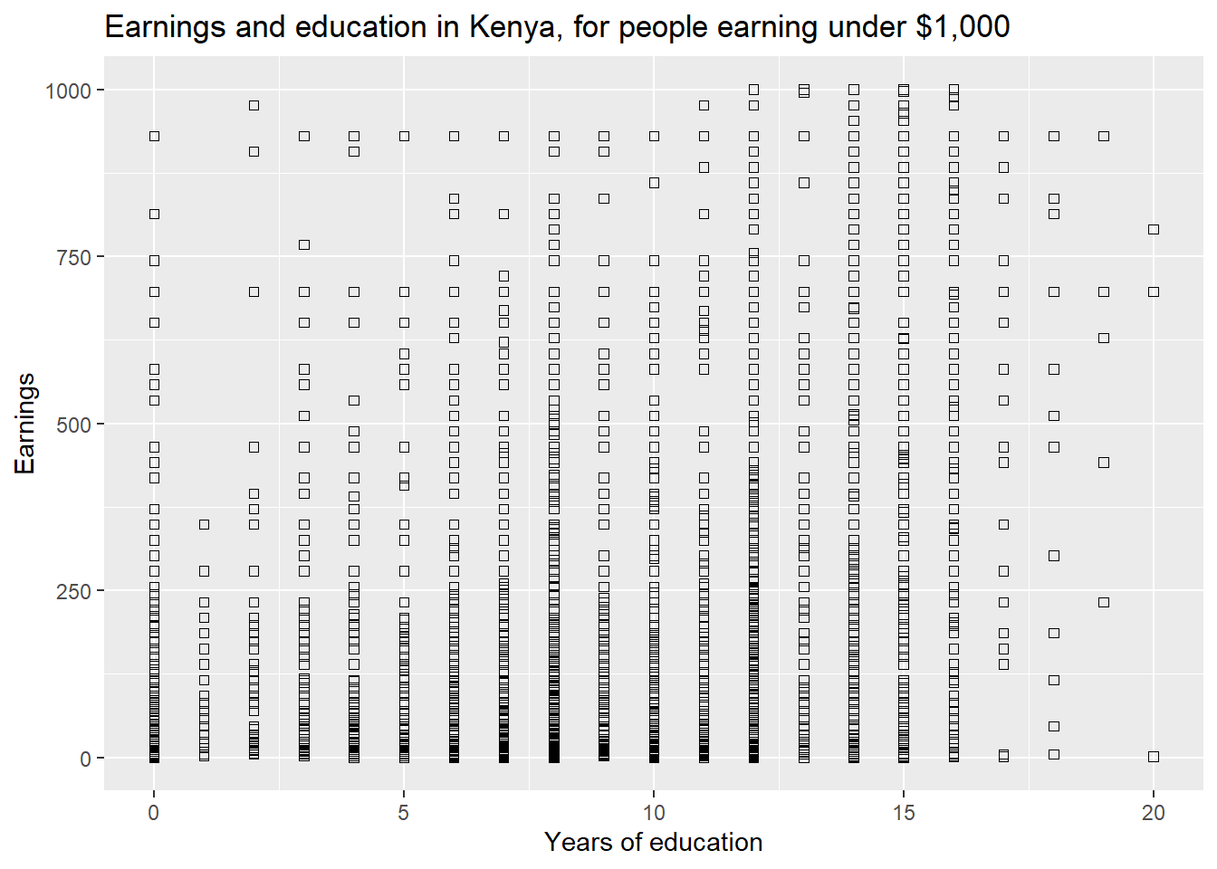
Additional scatter plot options can be used to generate even more infor- mative figures. For example, if you want to include a “best fit” line in the scatter plot. We will later (in Chapter 3) call this a regression line.
ggplot(data=subset(kenya,earnings_usd<=1000), aes(x=educ_yrs,y=earnings_usd)) +
geom_point(shape=0)+ labs(title="Earnings and education in Kenya, for people earning under $1,000") +
labs(x="Years of education", y="Earnings")+ geom_smooth(method=lm)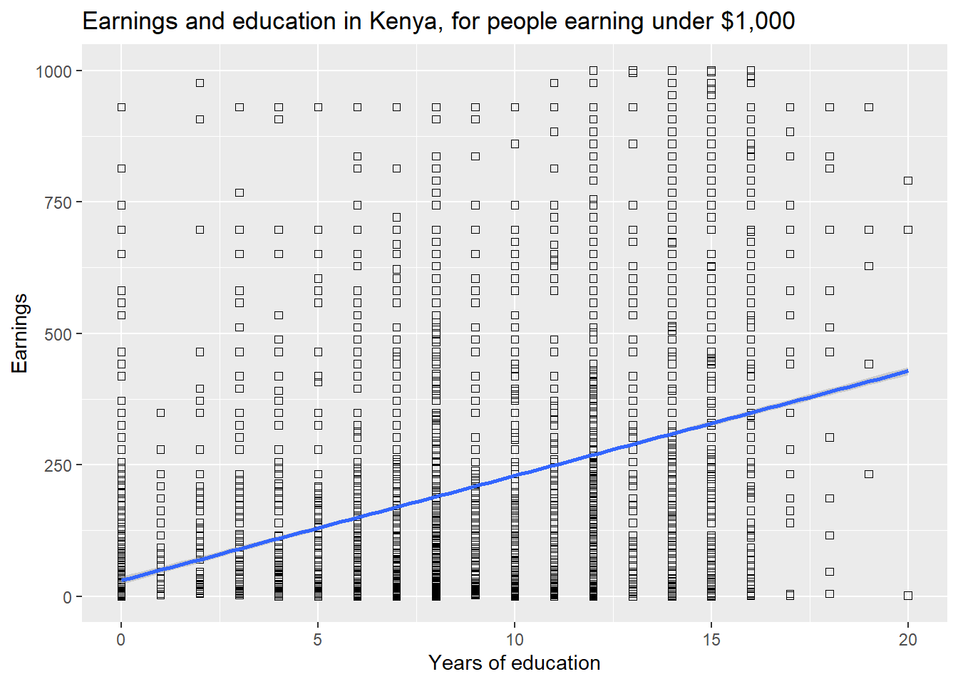
For a smoothed fitted curve, use geom smooth(method=loess).
12.7 Saving the script
Whenever you need to write a script, you can simply modify an existing script and then use the dropdown menu at the top to “Save as” and using a new filename or an updated filename reflecting the assignment or exercise (e.g. Chapter 2 script v3.R), where the v3 means this is version 3. It is good practice to not include special characters in a file name. These special characters include: %, #, &, etc.
Save your script frequently. There is no cost to repeatedly saving your script, and a huge cost to doing 5 hours of work without saving and have your computer suddenly crash perhaps because it ran out of battery power and so nothing is saved. So save frequently. We also recommend saving several versions by adding v1, v2, v3 to the file name as you do edits that are more extensive. Save your file using a descriptive name, not script.R or final script.R or final revised final script.R.