Chapter 13 Bootstrap in Modelling
In Chapter 11, we introduced the bootstrap, an exceptionally versatile technique. While it is often applied to estimate the standard deviation of a quantity when direct calculation is difficult or impossible, here we encounter it in a very different role: as a tool to enhance model estimation.
Motivation: Most tests related to model building (e.g. testing the significance of parameters) assumes normality and/or large samples. This is not always the case.
For example, in classical simple linear regression: the Gaussian model assumes that the errors are normally distributed. That is:
\[ y_i = \beta_0+\beta x_i +\varepsilon_i\\ \varepsilon_i \overset{iid}{\sim} N(0,\sigma^2) \]
This further implies the distribution of the OLS estimator has the following distribution:
\[ \hat{\beta} = \frac{\sum(y_i-\bar{y})(x_i-\bar{x})}{\sum(x_i-\bar{x})^2} \sim N\left(\beta,\frac{\sigma^2}{\sum(x_i-\bar{x})^2}\right) \]
And finally,
\[ \frac{\hat{\beta}-\beta}{\widehat{se(\hat{\beta})}} \sim t_{\nu = n-2} \]
where \(\widehat{se(\hat{\beta})}=\sqrt{MSE/\sum(x_i-\bar{x})^2}\)
Inferences about the coefficients \(\beta\) that are based on the T-distribution (e.g. confidence intervals and t-test p-values) will be invalid if the error terms are not normally distributed.
Bootstrap counterparts may be conducted when the data fail to meet these assumptions or data requirement.
13.1 Nonparametric Bootstrap Regression
IDEA: Make no parametric assumptions about the model — resample entire data pairs.
Suppose \(y_i\) is the value of the response for the \(i^{th}\) observation, and \(x_{ij}\) is the value of the \(j^{th}\) predictor for the \(i^{th}\) observation. In this example, \(y_i\)s are assumed to be independent such that:
\[ E(y_i|x_i) = \sum_{j=1}^px_{ij}\beta_j+\beta_0 \]
This means the data is cross-sectional, where rows are independent of each other.
Let’s say that the model being fitted is:
\[ y_i=\sum_{j=1}^p x_{ij}\beta_j+ \beta_0 +\varepsilon_i \]
where \(E(\varepsilon_i)=0\), \(Var(\varepsilon_i)=\sigma^2\), \(cov(\varepsilon_i,\varepsilon_j) = 0\)
Do the following to perform inference on \(\beta_j\) via nonparametric bootstrap:
Nonparametric Bootstrap for Regression Coefficient \(\beta_j\)
Input: Dataset \((y_1,\textbf{x}^T_1),...,(y_n,\textbf{x}^T_n)\)
Output: Inference on coefficient \(\beta_j\)
Take a simple random sample of size \(n\) with replacement from the data set.
\[ (y_1,\textbf{x}_1^T)^*,...,(y_n,\textbf{x}_n^T)^* \]
This is your bootstrap resample.
Using OLS (or whatever fitting procedure applies), fit a model, and compute the estimates \(\hat{\beta}_j^*\)
Repeat steps 1 and 2 \(B\) times. (\(B\) must be large)
Collect all \(B\) \(\hat{\beta}_j^*\)s and compute measures that apply.
For POINT estimation
The average of \(\hat{\beta}_j^*\)s is the bootstrap estimate
The estimated standard error is the standard deviation of the \(\hat{\beta}_j^*\)s
Note: the method of averaging the \(\hat{\beta}_j^*\)s is also referred as “Bagging” (See Section 13.3)
For INTERVAL estimation
The simplest approach for constructing a \((1 − \alpha)100\%\) Confidence Interval Estimate is using Percentiles.
\((P_{\alpha/2},P_{1-\alpha/2})\) where \(P_k\) is the \(k^{th}\) quantile.
For interval-based HYPOTHESIS TEST
The usual hypothesis is \(Ho: \beta_j=0\) vs \(Ha:\beta_j\neq0\)
You can use the computed C.I. estimate.
At \(\alpha\) level of significance, reject \(Ho\) when 0 is not in the \((1-\alpha)100\%\) interval estimate.
13.2 Semiparametric Bootstrap Regression
IDEA: Keep the model structure parametric, but resample the residuals nonparametrically.
The following is an algorithm that implements residual bootstrapping
Semiparametric Bootstrapping
Input: Dataset \((y_1,\textbf{x}^T_1),...,(y_n,\textbf{x}^T_n)\)
Output: Inference on coefficient \(\beta_j\)
Fit the model using the original data to obtain:
the coefficient estimates \(\hat{\beta}_0,\hat{\beta}_1,...,\hat{\beta}_k\)
the fitted values \(\hat{y}_i=\hat{\beta}_0 + \hat{\beta_1}x_{i1} + \cdots + \hat{\beta_k}x_{ik}\)
the residuals \(e_i=y_i-\hat{y}_i\)
From the residuals \((e_1,...,e_n)\), sample with replacement to obtain bootstrap residuals \((e_1^*,e_2^*,...e_n^*)\).
Using the resampled residuals, create a synthetic response variable \(y_i^*=\hat{y}_i+e_i^*\)
Using the synthetic response variable \(y_i^*\), refit the model to obtain bootstrap estimate of the coefficients \(\hat{\beta}_0^*,\hat{\beta}_1^*,\cdots,\hat{\beta}_k^*\)
Repeat 2,3,4 \(B\) times to obtain \(B\) values of \(\hat{\beta}_0^*,\hat{\beta}_1^*,\cdots,\hat{\beta}_k^*\)
Compute measures that apply (e.g. standard error, confidence intervals, etc…)
Interval Estimation and Hypothesis Test follow the same concept.
13.3 Bagging Algorithm
Bootstrap aggregating (or bagging) is a useful technique to improve the predictive performance of models, e.g., for additive models with high-dimensional predictors.
The idea is to generate several models via bootstrap and aggregate predicted values via averaging.
Bagging is commonly used to improve tree models or decision trees (such method is called random forest)
It is ideal for minimizing the instability or variance of a model in terms of prediction
The following are some examples of application of bagging.
Basic Bagging Algorithm for Predicted Values
Input: The dataset \((\textbf{y},\textbf{X})\). Note that each row is an independent observation.
Output: The “bagged” predicted value \(\hat{\textbf{y}}_{bag}\)
DO the following \(B\) times:
GENERATE a bootstrap sample \((\textbf{y}^*_b,\textbf{X}^*_b)\)
FIT a model \(\hat{f}(\textbf{X}_b^*)=\textbf{X}_b^*\hat{\boldsymbol{\beta}}_b\)
COMPUTE predicted value \(\widehat{\textbf{y}_b}=\textbf{X}_b^*\hat{\boldsymbol{\beta}}_b\)
END LOOP
COMPUTE “Bagged” predicted value \(\widehat{\textbf{y}}_{bag}=\frac{1}{B}\sum_{b=1}^B\widehat{\textbf{y}_b}\)
Random Permutations of Predictors
While Bagging focuses on resampling data, we can introduce additional randomness by randomly selecting or permuting predictors when training each model.
In this approach, you create many models where some models in the ensemble do not contain some predictors. This creates diversity among the models and enhances ensemble performance.
It appeals to relationships where the set of significant predictors vary across different “groups” or “types” of observation.
This allows computing the impact of a variable in the bagged predictive model.
The impact factor is usually computed as the difference of the expected prediction error of models that include the variable from those that do not include the variable.
Suggestions for Research using Bagging
explore bagging algorithm for a real predictive modeling task. (e.g. improve a linear model via bagging)
bagging algorithm for modeling high dimensional data (i.e. p >> n). Hence, only a subset of variables can be considered at a time.
design a strategic randomization method and/or aggregation strategy for Bagging a certain model.
explore the impact score as a tool for variable selection.
Exercise
Create a function boot_reg that implements residual bootstrap in simple linear regression. It should have the following parameters:
y- a vector of the dependent variablex- a vector of the independent variablealpha- the \(\alpha\) level of significanceB- the number of bootstrap replicates
It should have the following as output in a list:
reg_table: a data frame with the following layout: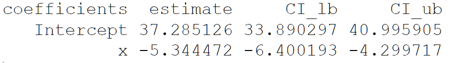
intercept_vec:vector of estimated coefficients \(\hat{\beta_0}^*\)betahat_vec: vector of estimated coefficients \(\hat{\beta}^*\)
Apply this function on the vectors mtcars$mpg and mtcars$wt as the dependent and independent variables respectively, with \(B = 2000\) and \(\alpha=0.05\)