Chapter 3 Assess MCMC Convergence And Evaluate HMSC Model Performance
Assessing Markov Chain Monte Carlo (MCMC) convergence in HMSC (Hierarchical Model of Species Communities) models is crucial because these models rely on MCMC sampling to estimate the posterior distributions of model parameters. If the MCMC algorithm has not converged, the posterior estimates may not be accurate or reliable. Convergence ensures that the MCMC chains have explored the parameter space sufficiently and are sampling from the true posterior distribution. If MCMC does not converge, the variance partitioning results might be unreliable, leading to incorrect identification of key drivers of community variation.
3.2 Load HMSC Model
VP_model_time_weather <- readRDS(paste0(here::here("Pollinator_Observations_HMSC_Workshop.rds")))3.3 Assess MCMC Convergence
The function convertToCodaObject in the HMSC package is used to convert the parameter estimates of a HMSC model into a format compatible with the coda package. The coda package provides tools for analyzing and diagnosing MCMC output, making it easier to assess convergence and explore posterior distributions.
VP_model_time_weather_convergence <- convertToCodaObject(VP_model_time_weather)3.3.1 How to Assess MCMC Convergence in HMSC
Effective Sample Size (ESS): The function
effectiveSizecalculates the effective sample size (ESS) of a MCMC chain. The ESS measures the number of independent samples in a MCMC chain. If the MCMC chain has high autocorrelation, the ESS will be much smaller than the actual number of samples (samplesargument in thesampleMcmcfunction), indicating poor mixing.Potential Scale Reduction Factor (PSRF): The PSRF compares the variance within chains to the variance between chains for each parameter. A PSRF close to 1 indicates that the chains have converged to the same distribution, meaning they have mixed well and are producing reliable estimates. A commonly accepted threshold is PSRF < 1.1.
VP_model_time_weather_convergence_ESS_PSRF <-
  data.frame(Trait = rep(colnames(VP_model_time_weather$Y), each = 8),
             Parameter = rep(c("B_Intercept",
                               "B_Time_Start_Decimal",
                               "B_SkyCloudy",
                               "B_SkyMostly_Clear",
                               "B_TemperatureHot",
                               "B_TemperatureWarm",
                               "B_WindNo",
                               "B_WindWindy"), 14),
             ESS = as.data.frame(effectiveSize(VP_model_time_weather_convergence$Beta))[, 1],
             Point_Est = as.data.frame(gelman.diag(VP_model_time_weather_convergence$Beta, multivariate = FALSE)$psrf)[, 1],
Upper_CI = as.data.frame(gelman.diag(VP_model_time_weather_convergence$Beta, multivariate = FALSE)$psrf)[, 2])VP_model_time_weather_convergence_ESS_PSRF## Trait Parameter ESS Point_Est Upper_CI
## 1 Bombus_Queen B_Intercept 1909.1788 1.0005678 1.0039293
## 2 Bombus_Queen B_Time_Start_Decimal 2076.1991 1.0031766 1.0128121
## 3 Bombus_Queen B_SkyCloudy 2000.0000 1.0028485 1.0151182
## 4 Bombus_Queen B_SkyMostly_Clear 1871.1112 1.0023720 1.0139903
## 5 Bombus_Queen B_TemperatureHot 2247.4086 1.0027787 1.0113331
## 6 Bombus_Queen B_TemperatureWarm 2000.0000 1.0034432 1.0185285
## 7 Bombus_Queen B_WindNo 2000.0000 0.9995562 0.9997324
## 8 Bombus_Queen B_WindWindy 2071.2852 1.0058700 1.0223404
## 9 Bombus_terrestris_Worker B_Intercept 869.2832 0.9995838 0.9995865
## 10 Bombus_terrestris_Worker B_Time_Start_Decimal 902.8207 1.0009605 1.0033081
## 11 Bombus_terrestris_Worker B_SkyCloudy 1612.8311 1.0026354 1.0083210
## 12 Bombus_terrestris_Worker B_SkyMostly_Clear 1251.1336 1.0077239 1.0361283
## 13 Bombus_terrestris_Worker B_TemperatureHot 2000.0000 1.0052372 1.0260360
## 14 Bombus_terrestris_Worker B_TemperatureWarm 1707.2304 1.0204776 1.0891957
## 15 Bombus_terrestris_Worker B_WindNo 1258.8041 1.0031805 1.0136244
## 16 Bombus_terrestris_Worker B_WindWindy 1837.8629 1.0285919 1.1291906
## 17 Bombus_Worker B_Intercept 2000.0000 1.0015035 1.0090894
## 18 Bombus_Worker B_Time_Start_Decimal 2015.2695 1.0042519 1.0218668
## 19 Bombus_Worker B_SkyCloudy 1798.4410 1.0039625 1.0216504
## 20 Bombus_Worker B_SkyMostly_Clear 1717.6885 1.0059854 1.0315655
## 21 Bombus_Worker B_TemperatureHot 1886.9348 1.0056875 1.0240556
## 22 Bombus_Worker B_TemperatureWarm 2000.0000 1.0010658 1.0078962
## 23 Bombus_Worker B_WindNo 2000.0000 0.9997290 0.9997322
## 24 Bombus_Worker B_WindWindy 2094.1973 1.0003551 1.0017606
## 25 Bombyliidae B_Intercept 1729.7435 0.9999723 1.0019343
## 26 Bombyliidae B_Time_Start_Decimal 1724.8357 1.0008475 1.0066325
## 27 Bombyliidae B_SkyCloudy 1849.8874 1.0257998 1.1181779
## 28 Bombyliidae B_SkyMostly_Clear 1406.2530 1.0091465 1.0434604
## 29 Bombyliidae B_TemperatureHot 2000.0000 1.0166737 1.0739374
## 30 Bombyliidae B_TemperatureWarm 2000.0000 1.0003985 1.0040256
## 31 Bombyliidae B_WindNo 1345.0012 1.0000359 1.0005294
## 32 Bombyliidae B_WindWindy 2000.0000 1.0089108 1.0445132
## 33 Coleoptera B_Intercept 1860.7534 1.0014410 1.0065152
## 34 Coleoptera B_Time_Start_Decimal 1887.3712 1.0006453 1.0007378
## 35 Coleoptera B_SkyCloudy 1730.0963 0.9999769 1.0018782
## 36 Coleoptera B_SkyMostly_Clear 2000.0000 1.0063649 1.0172315
## 37 Coleoptera B_TemperatureHot 2000.0000 1.0120066 1.0584262
## 38 Coleoptera B_TemperatureWarm 2000.0000 1.0188058 1.0860962
## 39 Coleoptera B_WindNo 2000.0000 1.0012299 1.0065817
## 40 Coleoptera B_WindWindy 2274.9394 1.0031960 1.0172441
## 41 Diurnal_Lepidoptera B_Intercept 1438.5444 1.0006290 1.0056104
## 42 Diurnal_Lepidoptera B_Time_Start_Decimal 1428.5061 0.9995906 1.0000534
## 43 Diurnal_Lepidoptera B_SkyCloudy 1860.9370 0.9999362 1.0023472
## 44 Diurnal_Lepidoptera B_SkyMostly_Clear 1372.9863 1.0119804 1.0460125
## 45 Diurnal_Lepidoptera B_TemperatureHot 2687.7910 1.0526548 1.2200053
## 46 Diurnal_Lepidoptera B_TemperatureWarm 1705.6259 1.0013978 1.0047647
## 47 Diurnal_Lepidoptera B_WindNo 1601.1400 1.0099760 1.0442102
## 48 Diurnal_Lepidoptera B_WindWindy 1807.0352 1.0506589 1.2106226
## 49 Honeybee B_Intercept 1556.5772 1.0015389 1.0102635
## 50 Honeybee B_Time_Start_Decimal 1643.3551 0.9998535 1.0019398
## 51 Honeybee B_SkyCloudy 1881.2638 1.0027908 1.0120422
## 52 Honeybee B_SkyMostly_Clear 1853.5957 1.0034395 1.0194396
## 53 Honeybee B_TemperatureHot 1909.6943 1.0040129 1.0195507
## 54 Honeybee B_TemperatureWarm 1900.8789 1.0064003 1.0327318
## 55 Honeybee B_WindNo 1830.0251 1.0022493 1.0095084
## 56 Honeybee B_WindWindy 1699.9384 1.0048307 1.0253836
## 57 Large_Solitary_Bee B_Intercept 2000.0000 0.9997378 1.0012482
## 58 Large_Solitary_Bee B_Time_Start_Decimal 2000.0000 0.9994274 0.9995252
## 59 Large_Solitary_Bee B_SkyCloudy 1603.8793 1.0072673 1.0359558
## 60 Large_Solitary_Bee B_SkyMostly_Clear 1888.6519 1.0042195 1.0231575
## 61 Large_Solitary_Bee B_TemperatureHot 2498.8561 1.0017325 1.0077558
## 62 Large_Solitary_Bee B_TemperatureWarm 1847.6009 1.0035462 1.0109748
## 63 Large_Solitary_Bee B_WindNo 1850.5399 1.0121023 1.0584854
## 64 Large_Solitary_Bee B_WindWindy 2000.0000 0.9993664 0.9994420
## 65 Noctuidae B_Intercept 2000.0000 1.0078989 1.0383988
## 66 Noctuidae B_Time_Start_Decimal 1848.7155 1.0028295 1.0161051
## 67 Noctuidae B_SkyCloudy 1741.7645 1.0009598 1.0041336
## 68 Noctuidae B_SkyMostly_Clear 2000.0000 1.0055479 1.0295401
## 69 Noctuidae B_TemperatureHot 2000.0000 1.0108732 1.0414256
## 70 Noctuidae B_TemperatureWarm 2000.0000 1.0148383 1.0718474
## 71 Noctuidae B_WindNo 1898.9181 1.0183699 1.0828026
## 72 Noctuidae B_WindWindy 1723.1922 1.0221623 1.1023655
## 73 Non_Syrphid_Diptera B_Intercept 2000.0000 0.9996475 1.0008467
## 74 Non_Syrphid_Diptera B_Time_Start_Decimal 1808.6414 0.9997822 0.9997837
## 75 Non_Syrphid_Diptera B_SkyCloudy 2000.0000 1.0000028 1.0004520
## 76 Non_Syrphid_Diptera B_SkyMostly_Clear 1621.6010 1.0001771 1.0006404
## 77 Non_Syrphid_Diptera B_TemperatureHot 2000.0000 1.0078205 1.0355664
## 78 Non_Syrphid_Diptera B_TemperatureWarm 2000.0000 1.0019310 1.0093977
## 79 Non_Syrphid_Diptera B_WindNo 2000.0000 1.0022954 1.0051974
## 80 Non_Syrphid_Diptera B_WindWindy 2000.0000 1.0043979 1.0229699
## 81 Other B_Intercept 2000.0000 1.0067798 1.0341738
## 82 Other B_Time_Start_Decimal 2155.9559 1.0021823 1.0112324
## 83 Other B_SkyCloudy 1529.7822 1.0024354 1.0140522
## 84 Other B_SkyMostly_Clear 2114.9363 1.0006338 1.0032425
## 85 Other B_TemperatureHot 1535.9474 1.0264916 1.1174531
## 86 Other B_TemperatureWarm 2095.3764 1.0083937 1.0426679
## 87 Other B_WindNo 1907.5276 1.0007868 1.0032460
## 88 Other B_WindWindy 2000.0000 1.0056774 1.0236794
## 89 Small_Solitary_Bee B_Intercept 1731.8422 1.0020998 1.0056642
## 90 Small_Solitary_Bee B_Time_Start_Decimal 1746.0341 1.0046434 1.0069856
## 91 Small_Solitary_Bee B_SkyCloudy 1875.0647 1.0006736 1.0033033
## 92 Small_Solitary_Bee B_SkyMostly_Clear 1773.8046 1.0101533 1.0458068
## 93 Small_Solitary_Bee B_TemperatureHot 2000.0000 1.0024184 1.0138026
## 94 Small_Solitary_Bee B_TemperatureWarm 2000.0000 0.9998096 1.0017179
## 95 Small_Solitary_Bee B_WindNo 1773.0716 1.0134270 1.0604567
## 96 Small_Solitary_Bee B_WindWindy 2000.0000 1.0290361 1.1092574
## 97 Sphingidae B_Intercept 2000.0000 1.0004790 1.0041370
## 98 Sphingidae B_Time_Start_Decimal 2000.0000 1.0001515 1.0033874
## 99 Sphingidae B_SkyCloudy 1884.4424 1.0036208 1.0097688
## 100 Sphingidae B_SkyMostly_Clear 2000.0000 1.0017594 1.0104994
## 101 Sphingidae B_TemperatureHot 2000.0000 1.0021089 1.0127270
## 102 Sphingidae B_TemperatureWarm 1628.5870 0.9998605 1.0012767
## 103 Sphingidae B_WindNo 2000.0000 0.9994842 0.9996903
## 104 Sphingidae B_WindWindy 2000.0000 1.0019040 1.0100071
## 105 Syrphidae B_Intercept 1779.7756 1.0011093 1.0080762
## 106 Syrphidae B_Time_Start_Decimal 1878.2614 0.9994690 0.9995593
## 107 Syrphidae B_SkyCloudy 1996.6888 1.0000601 1.0029214
## 108 Syrphidae B_SkyMostly_Clear 2000.0000 0.9995766 1.0002913
## 109 Syrphidae B_TemperatureHot 1669.0577 1.0265390 1.1207036
## 110 Syrphidae B_TemperatureWarm 2000.0000 1.0110894 1.0550612
## 111 Syrphidae B_WindNo 1575.9999 1.0110614 1.0547197
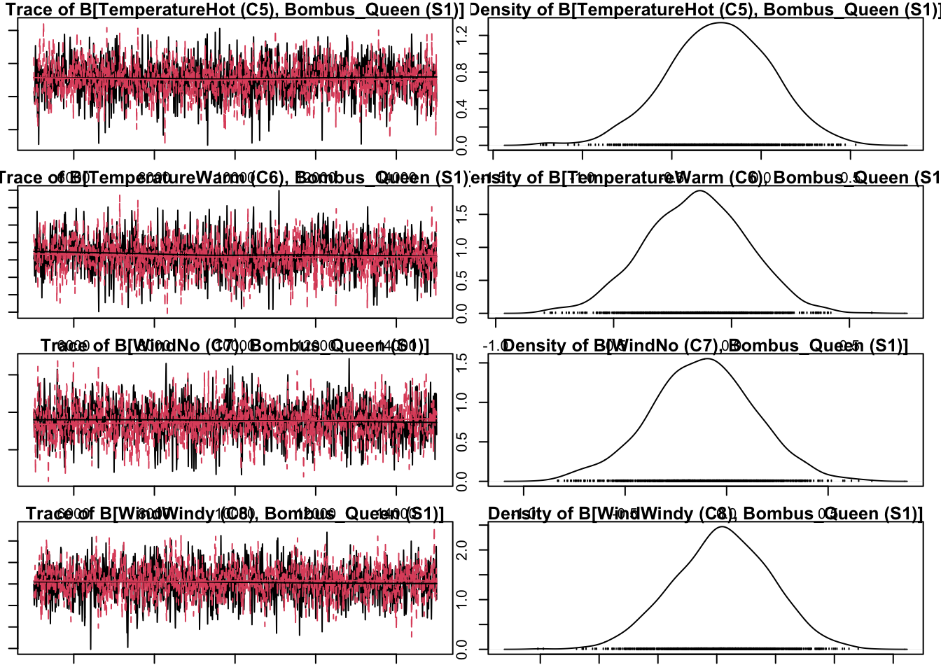
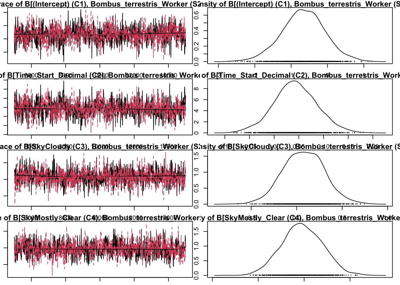
## 112 Syrphidae B_WindWindy 2000.0000 1.0021323 1.00829013.4 Posterior Trace Plots
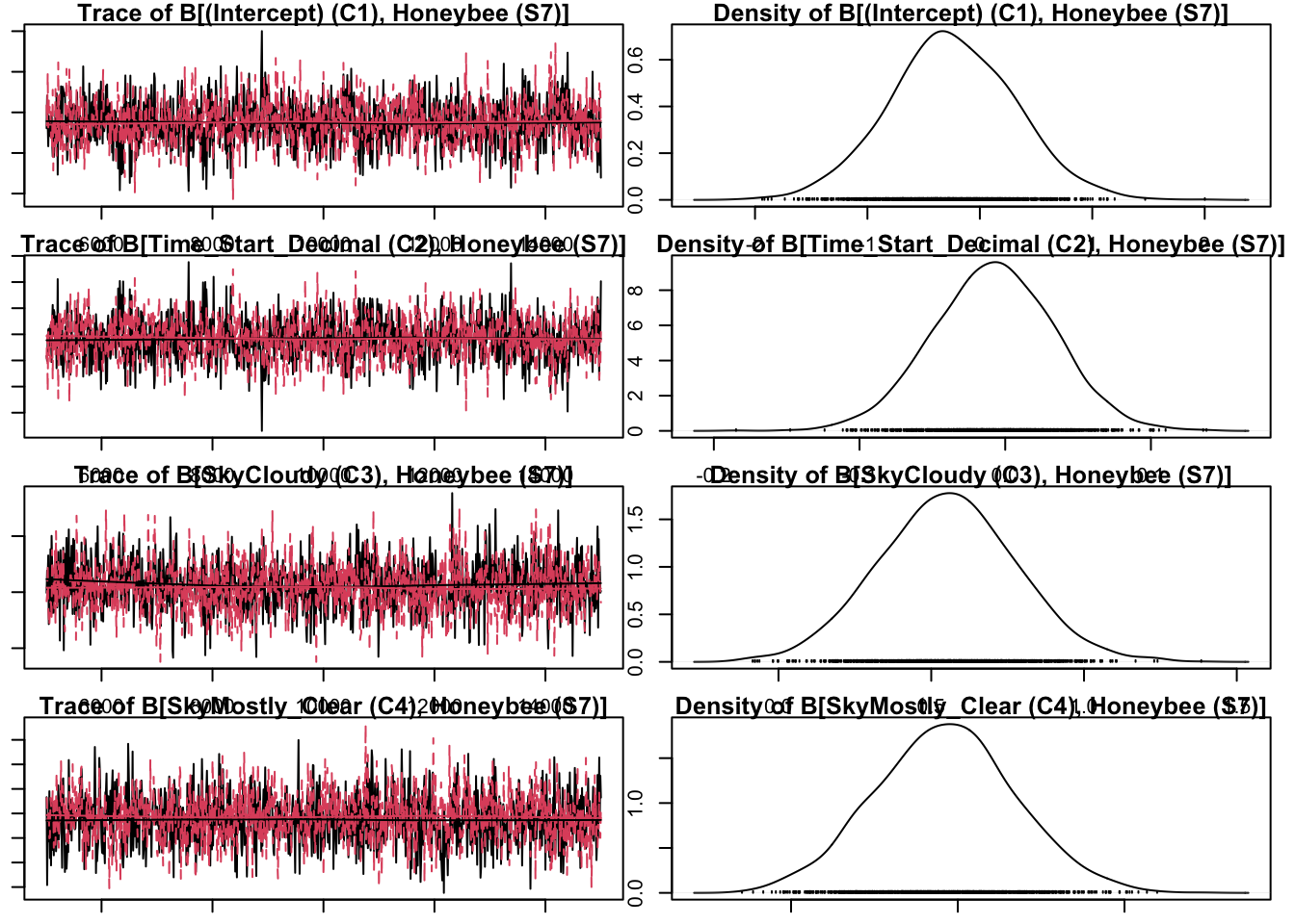
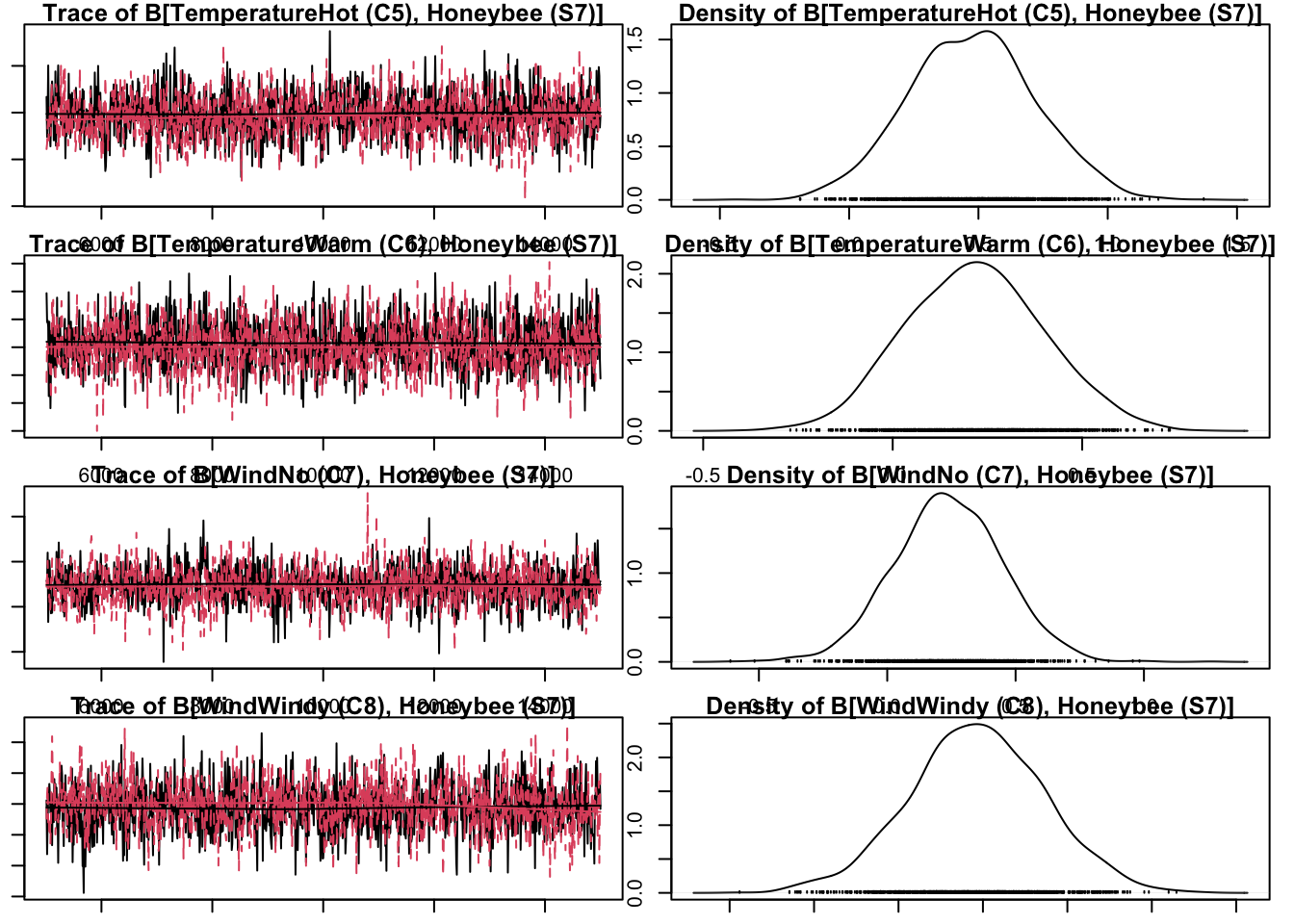
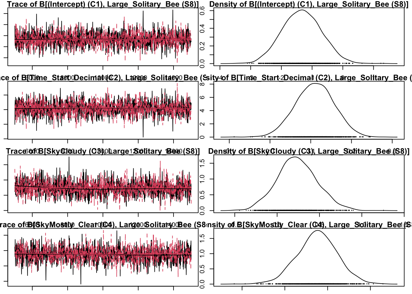
Posterior trace plots are a key visual diagnostic tool to assess the convergence of MCMC. These plots show how the sampled values of a parameter change across iterations of the MCMC algorithm. Trace plots are especially helpful for identifying problems such as poor mixing or lack of stationarity in the chains, which indicate that the MCMC has not converged.
3.4.1 How to Assess MCMC Convergence in HMSC
Well-Mixed Chains: The chains rapidly rise and fall (i.e. they jump freely across the plot).
Stationarity: The chains should wander around a stable mean with no obvious trends.
Consistency Across Chains: If multiple chains are run, their trace plots should overlap and look similar, suggesting that they have converged.
par(mar = c(1, 1, 1, 1))

plot(VP_model_time_weather_convergence$Beta)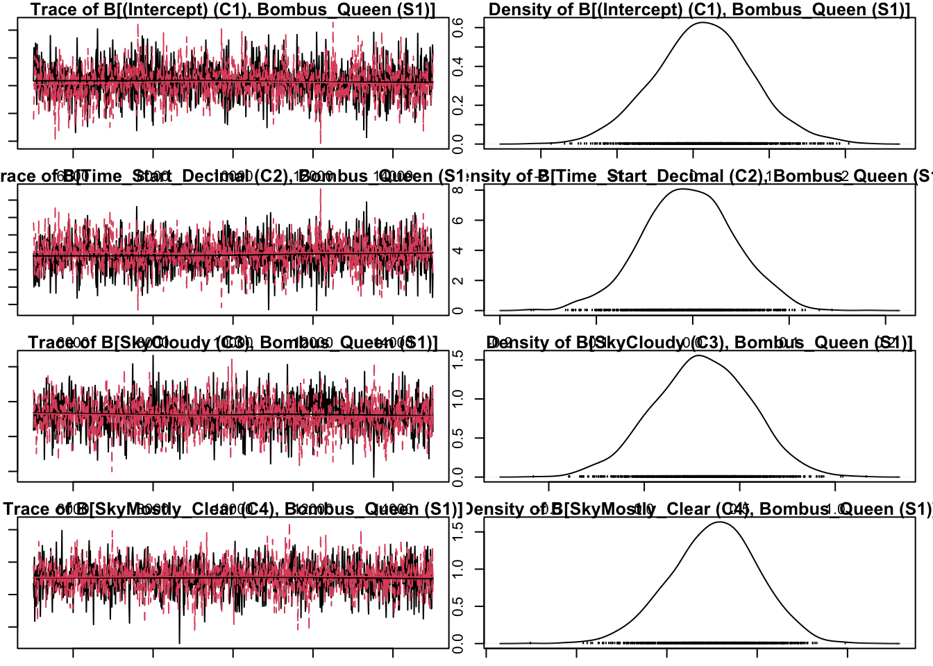
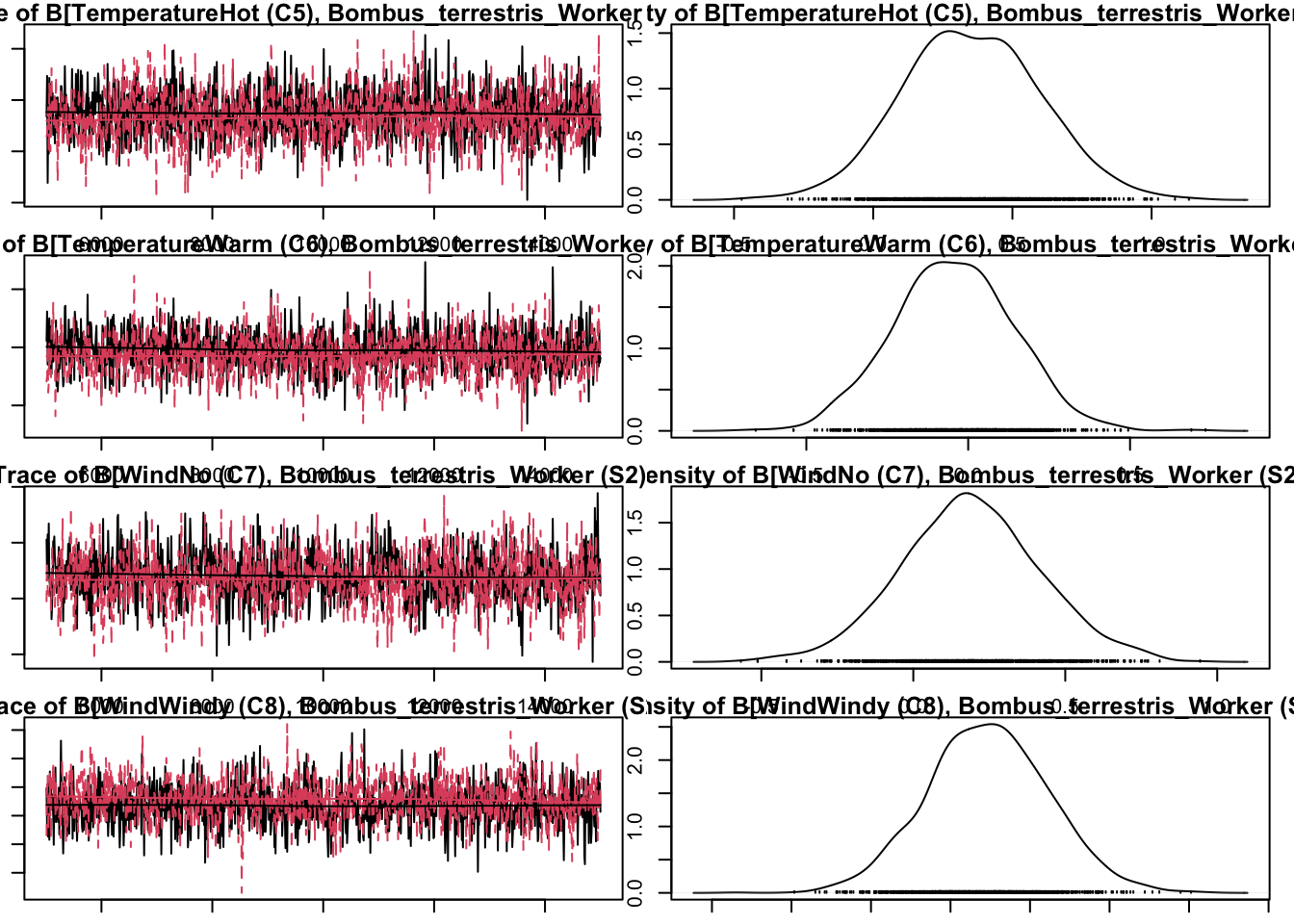
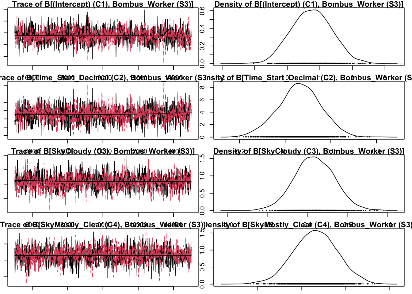
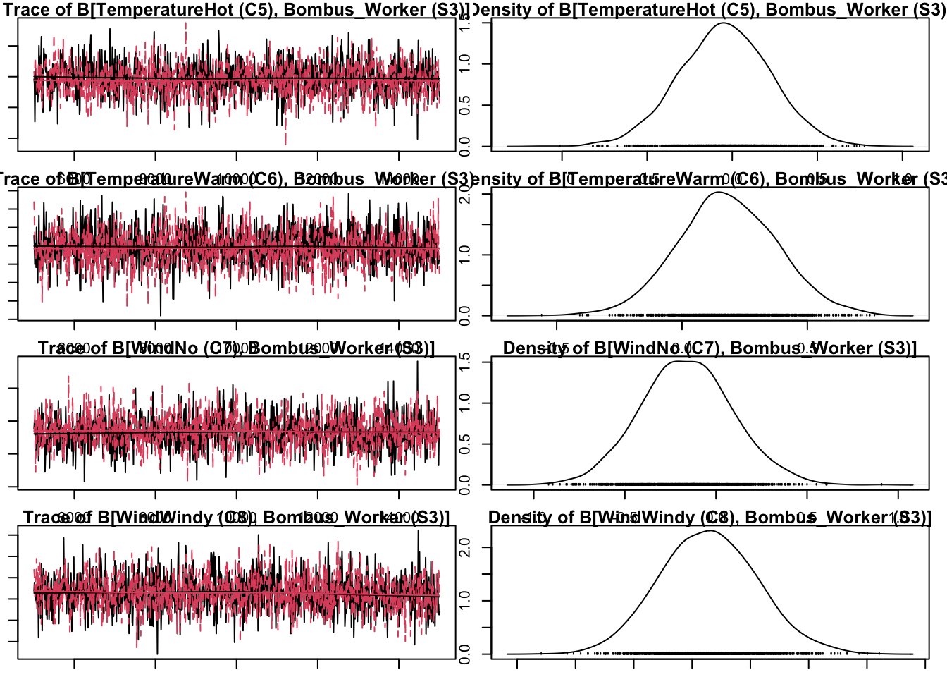
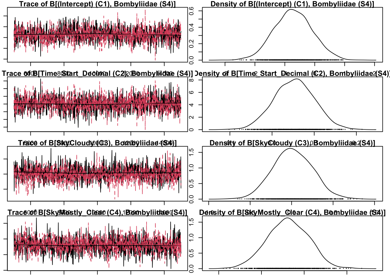
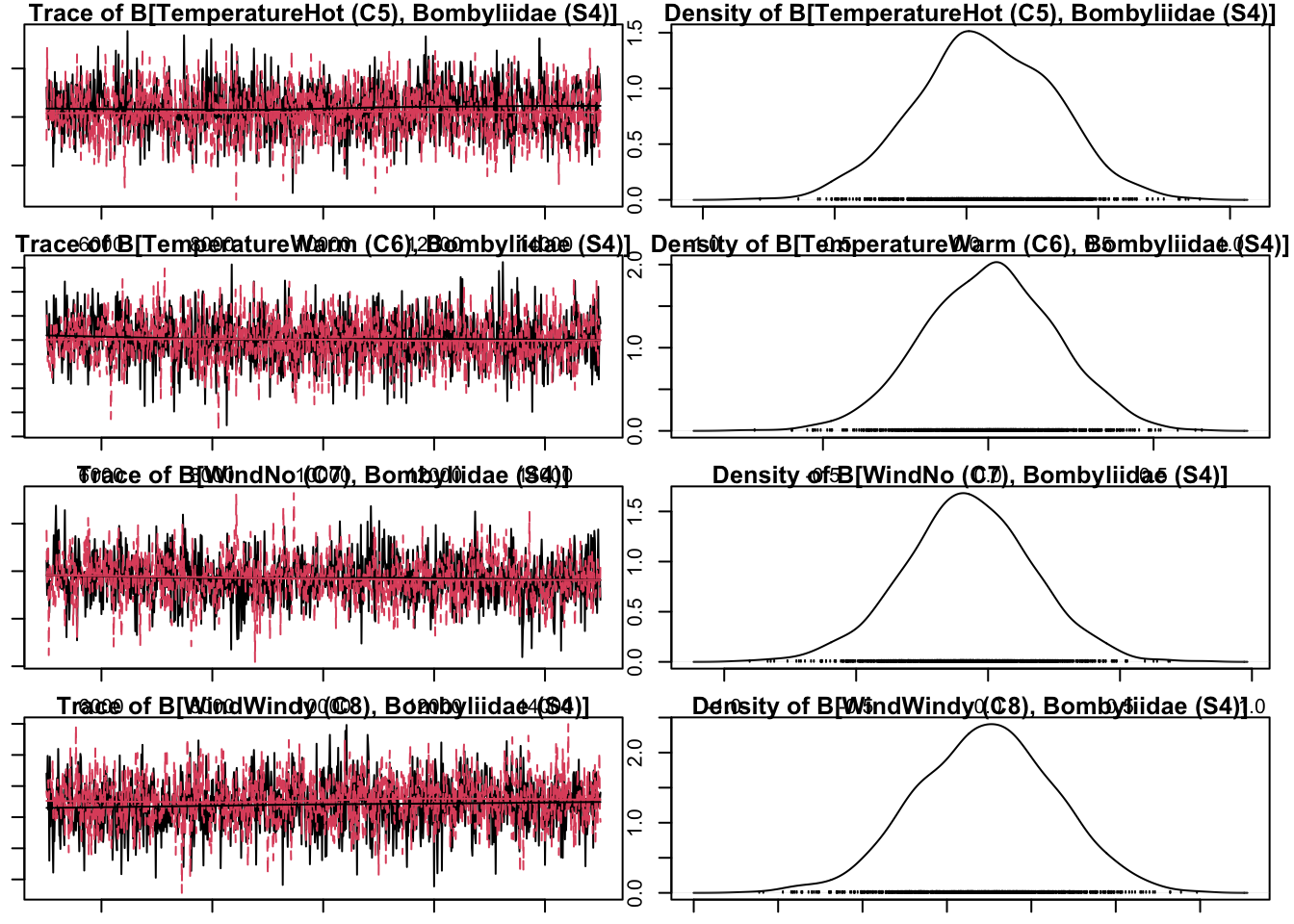
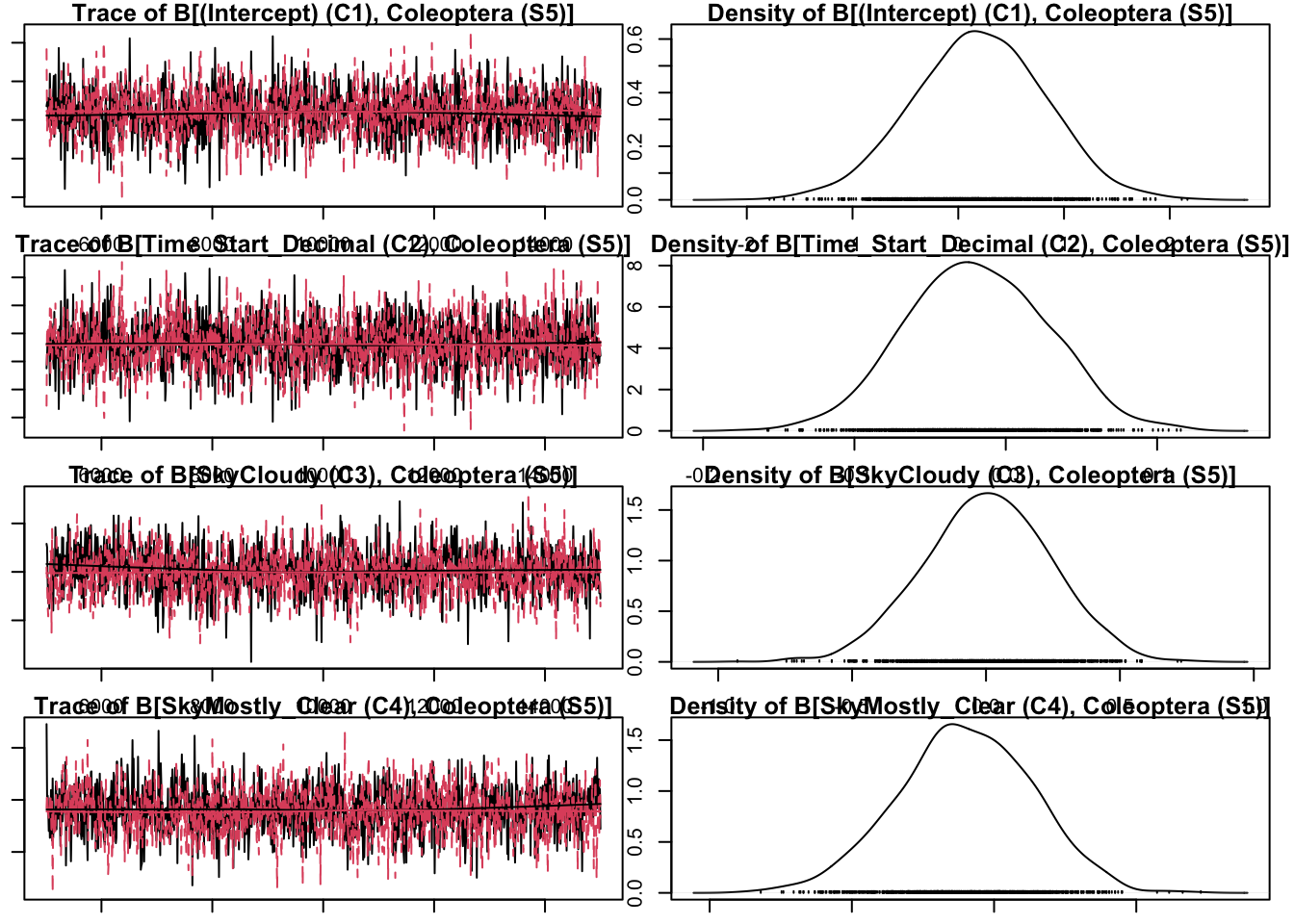
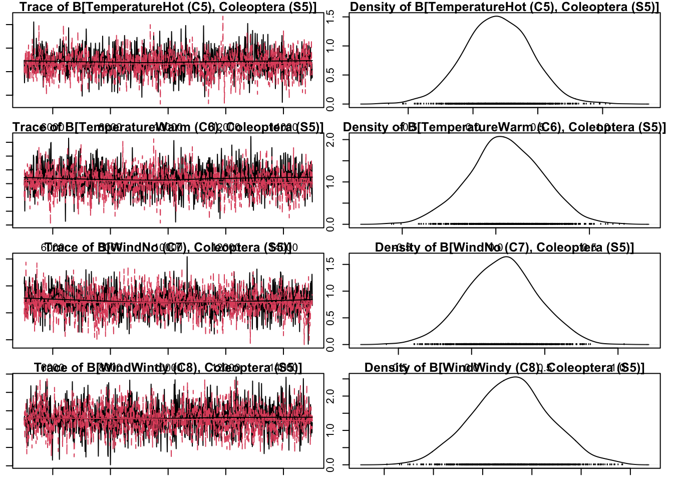
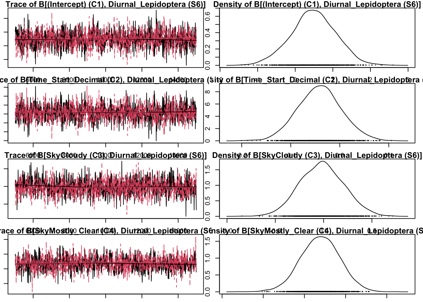
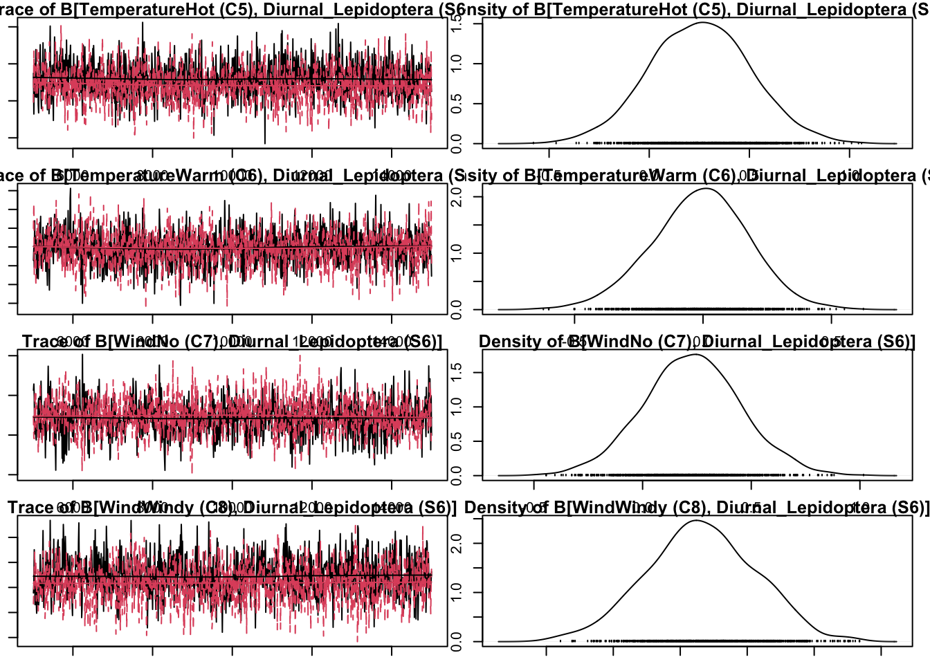
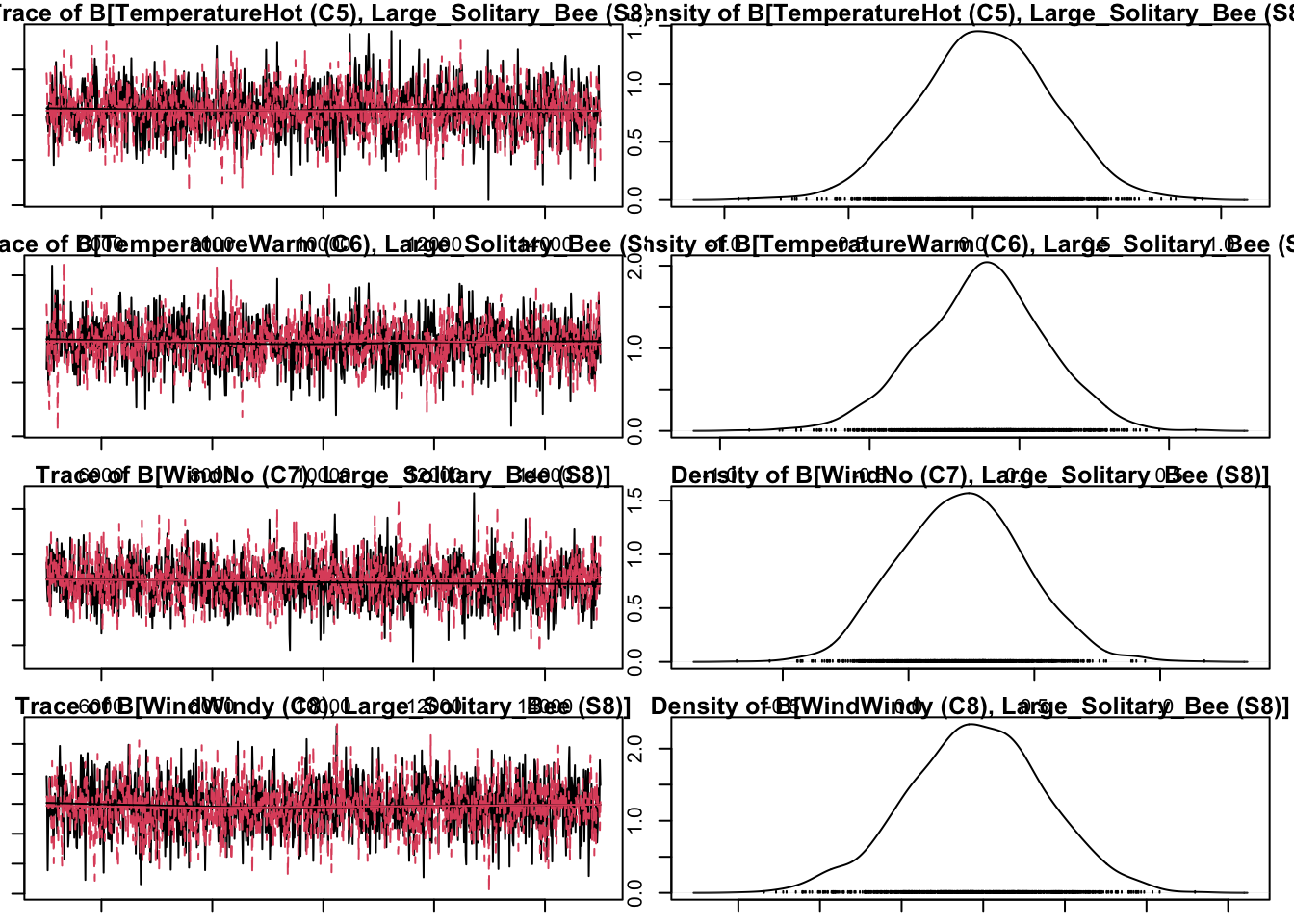
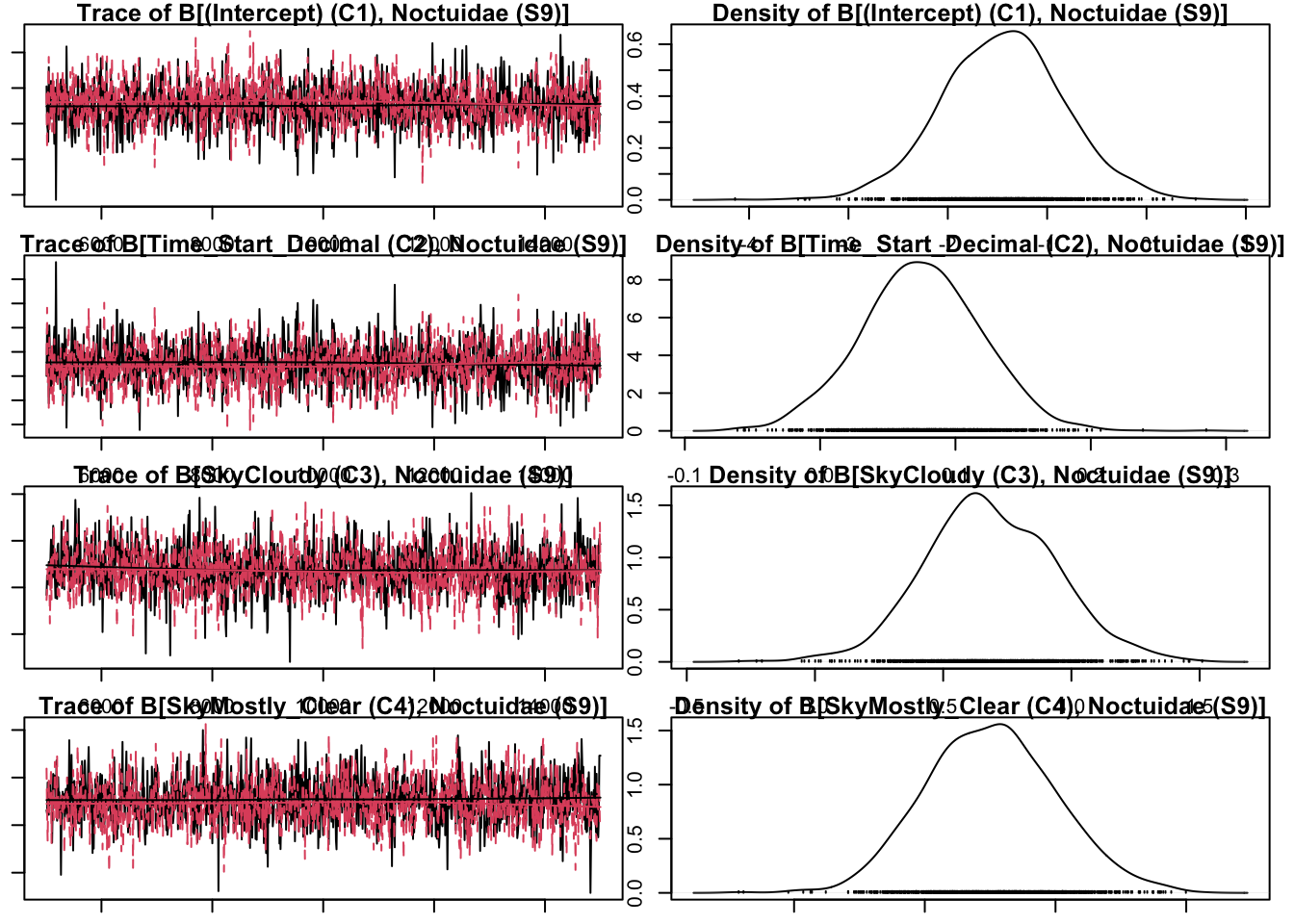
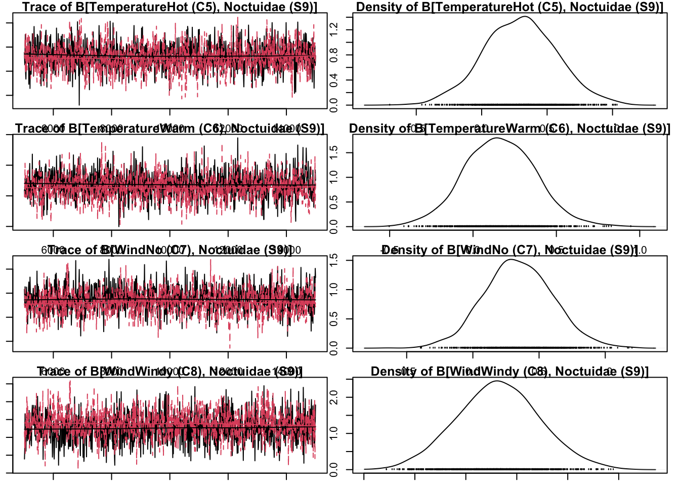
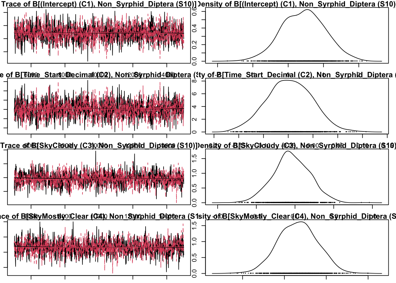
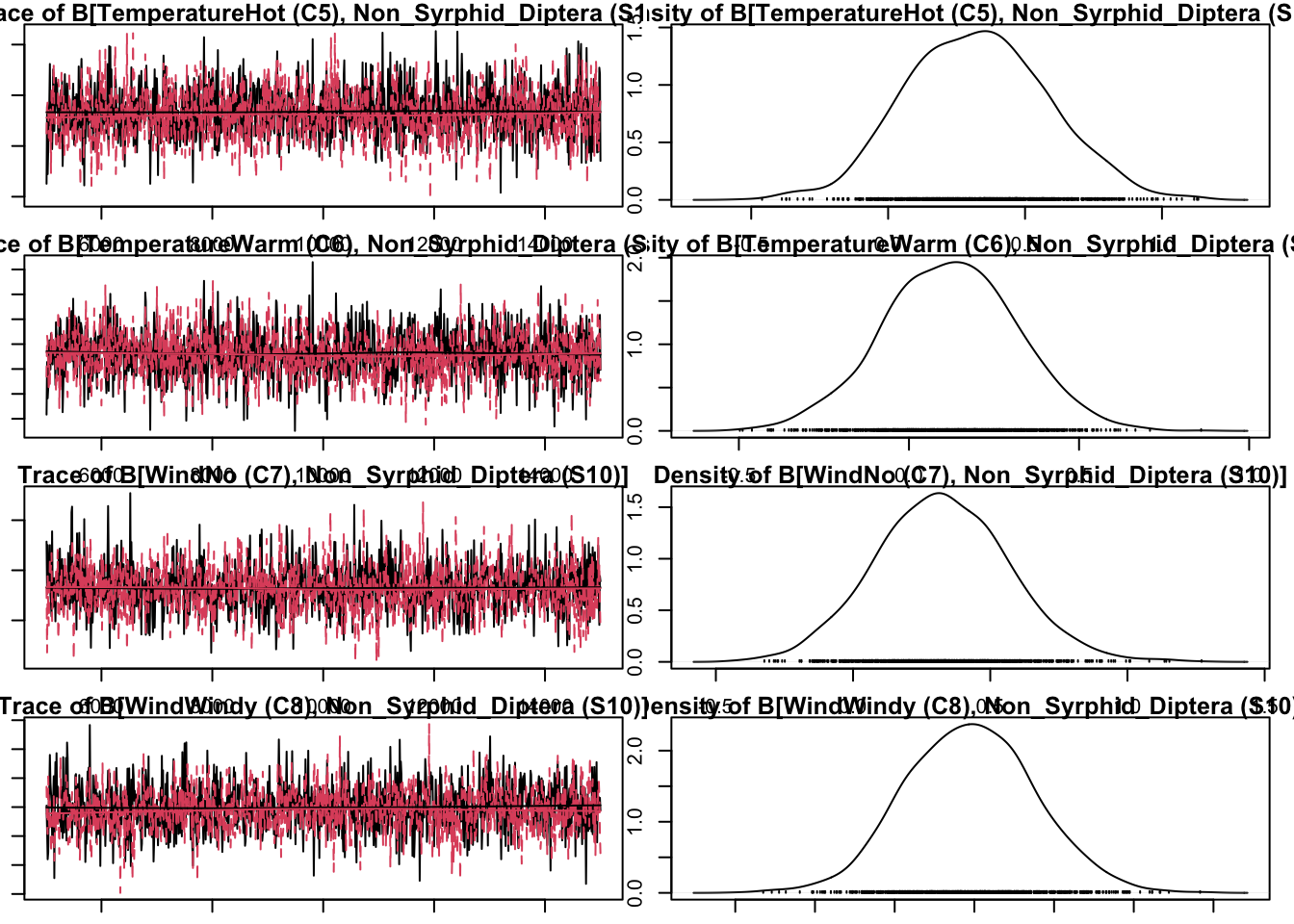
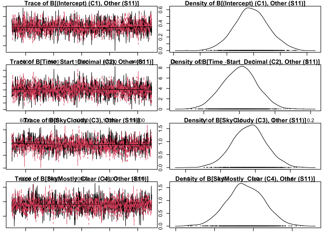
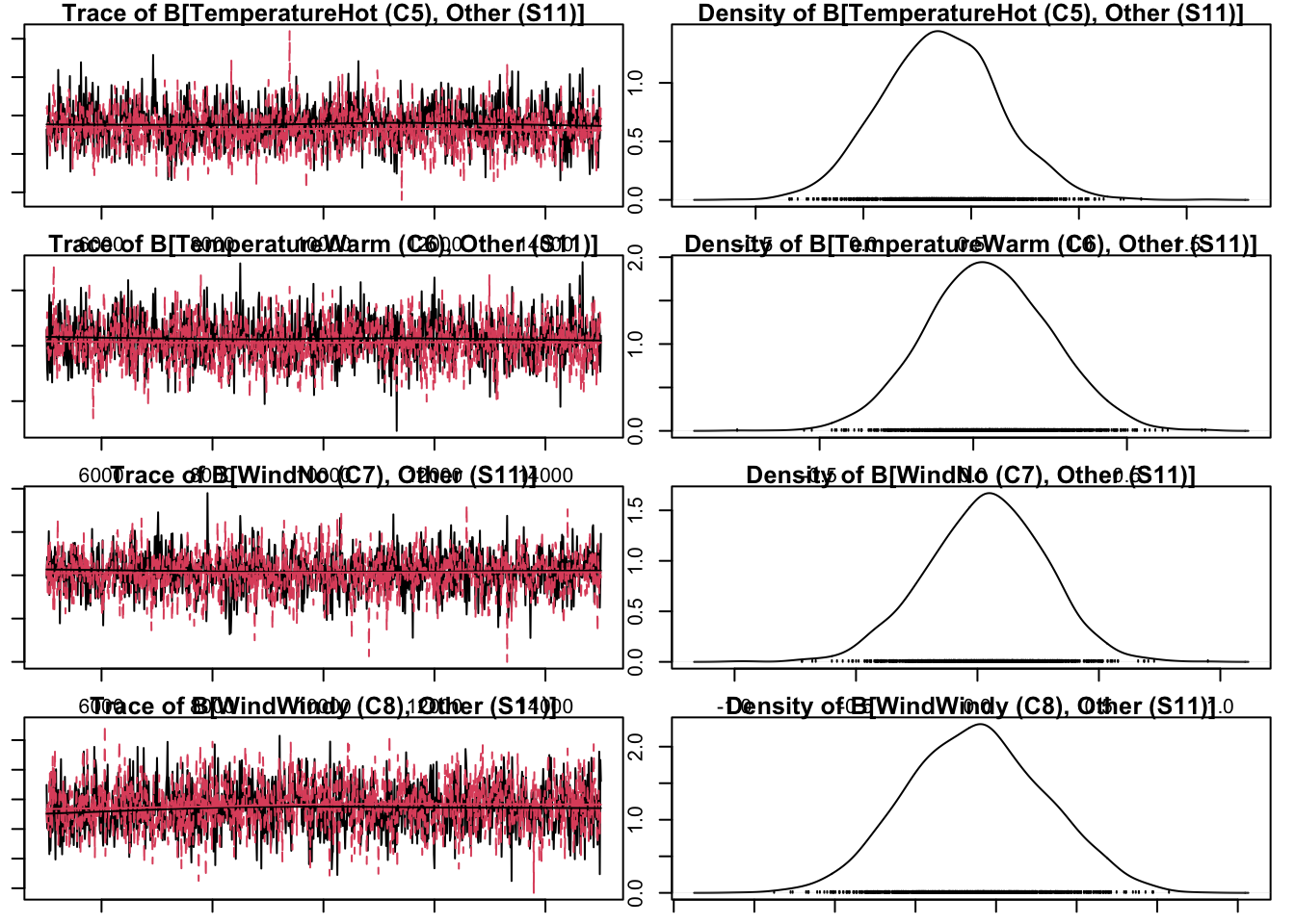
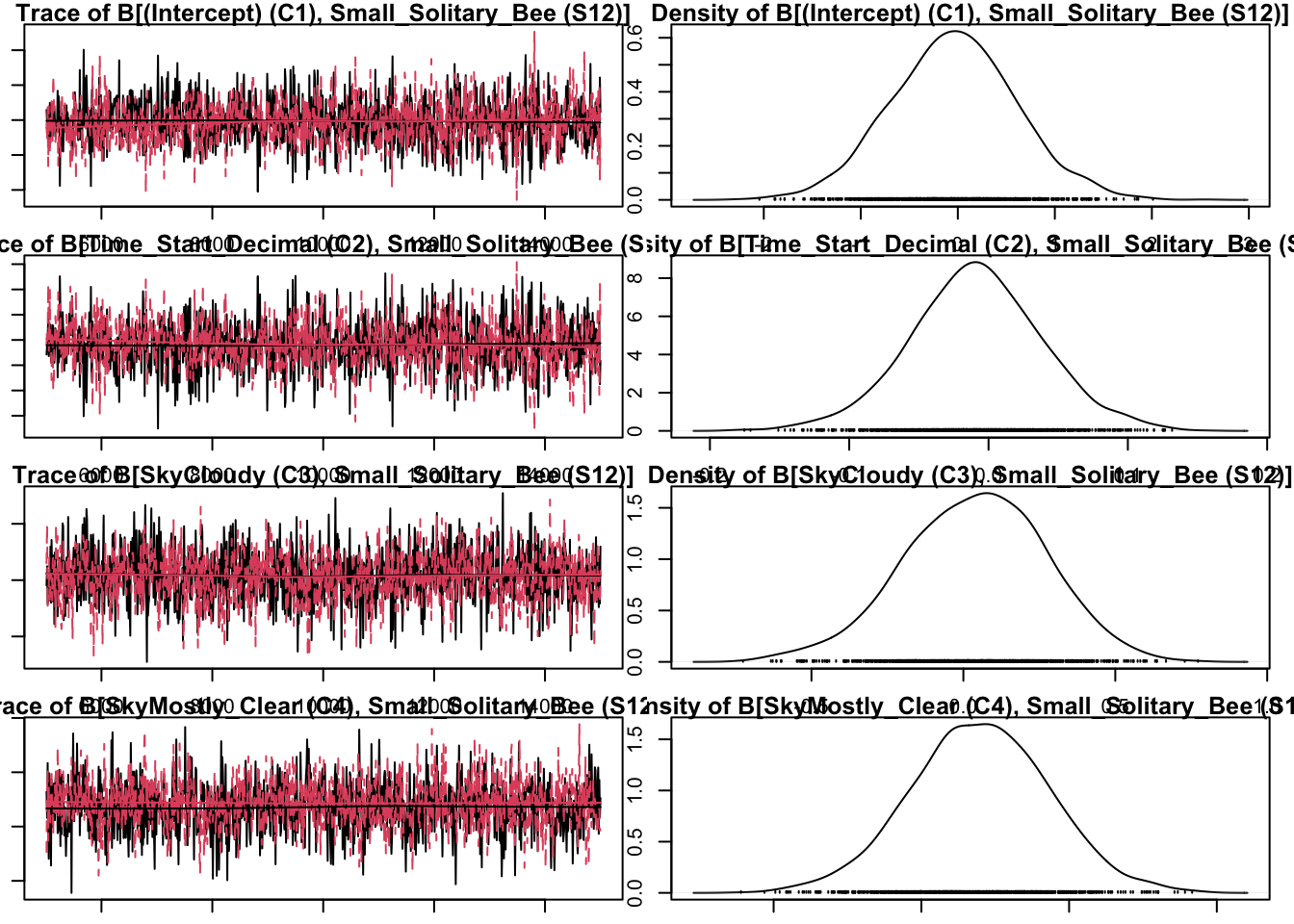
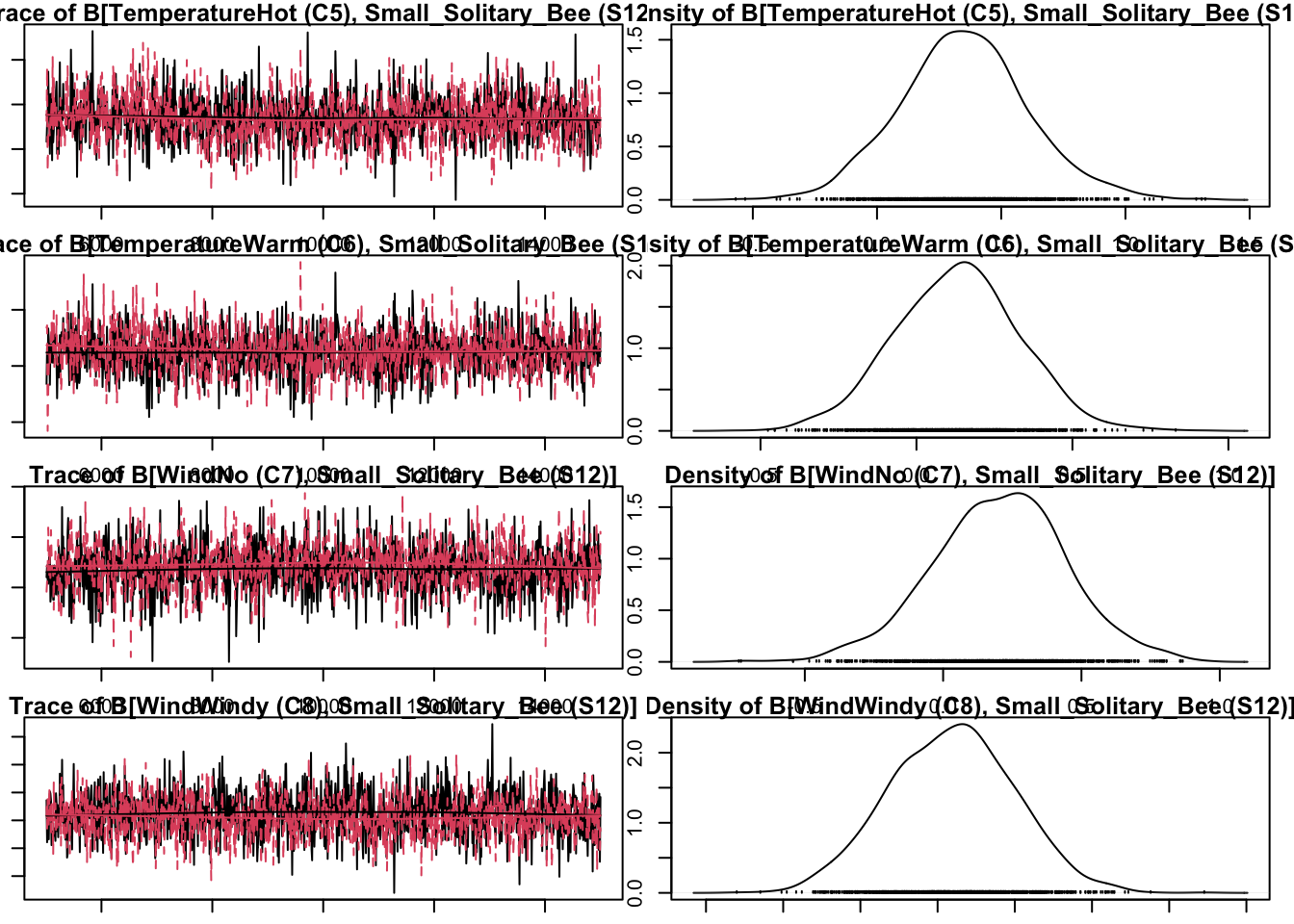
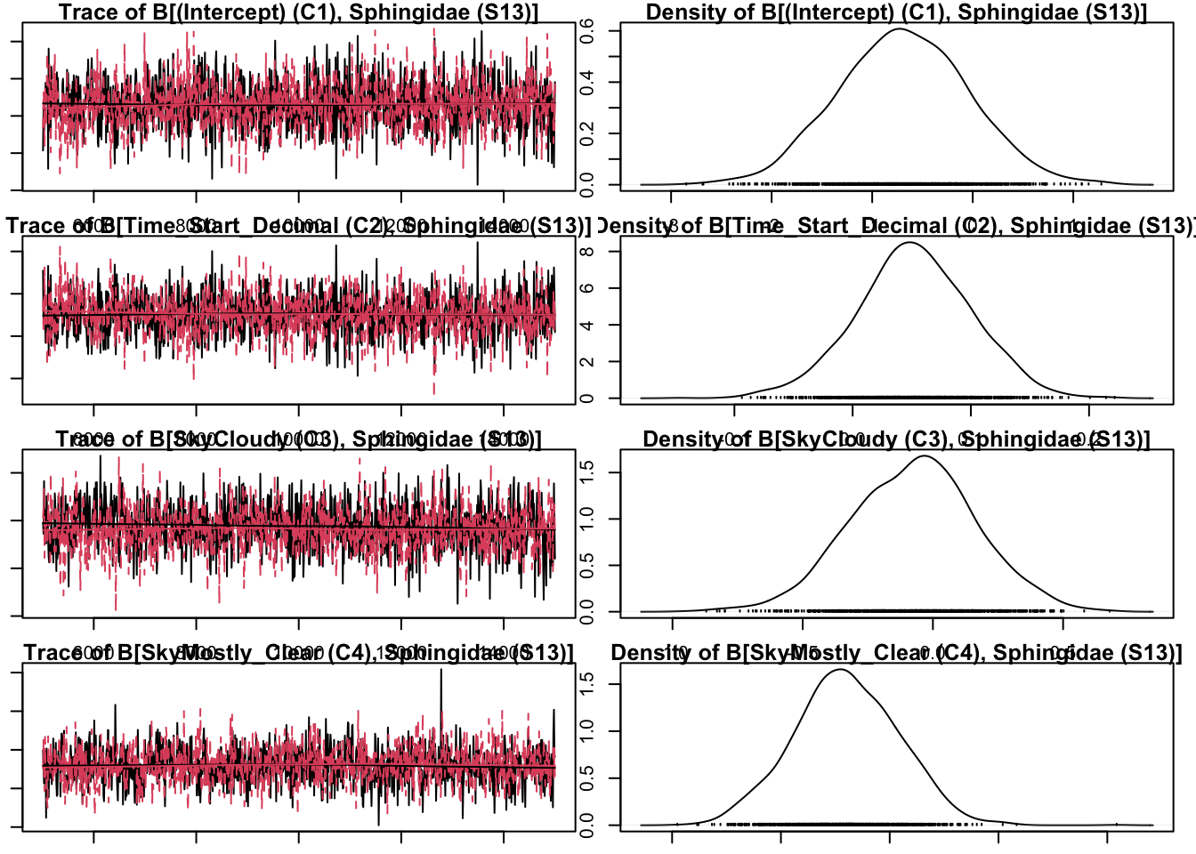
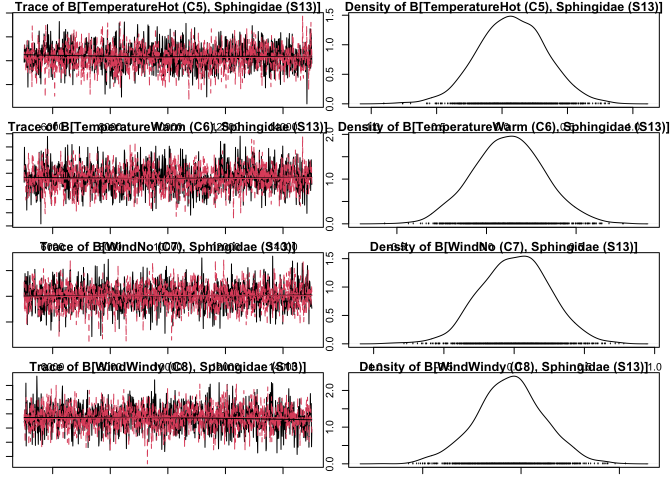
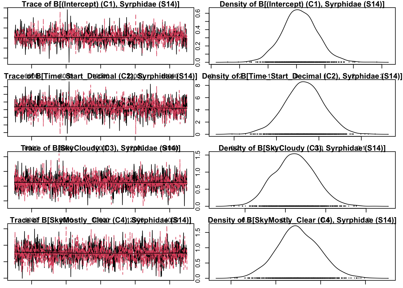
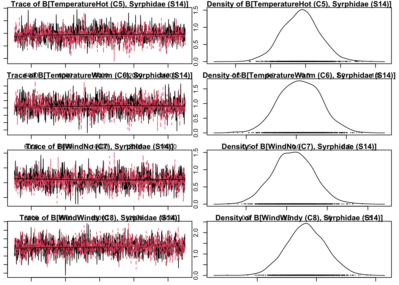
If the MCMC convergence is not satisfactory, it is then necessary to re-fit the HMSC model using different parameter values (samples, thin, and transient arguments of the function sampleMcmc). If the posterior trace plots indicate inadequate chain mixing or obvious trends, it is recommended to increase the value of the transient argument (i.e. increase burn-in period). If the chains indicate autocorrelation and differ from each other, it is recommended to increase the value of the thin argument, while keeping the samples argument fixed.
3.5 HMSC Model Performance
The Root Mean Squared Error (RMSE) and R² (coefficient of determination) are key metrics for assessing the performance of HMSC models. These metrics provide insights into how well the model explains variation in the response variables (e.g. species abundances or occurrences). It is important to evaluate RMSE and R² for each species to identify which species are well-predicted and which are not.
What RMSE Tells You: A lower RMSE indicates better model performance, as predictions are closer to the observed values. RMSE measures the average error between observed values and the model’s predicted values.
What R² Tells You: R² measures the proportion of variance in the observed data that is explained by the model. R² = 1 represents a perfect fit, meaning the model explains 100% of the variance in the observed data.
VP_model_time_weather_predicted_values <- computePredictedValues(VP_model_time_weather, expected = FALSE)VP_model_time_weather_performance_RMSE_R2 <-
data.frame(Variable = colnames(VP_model_time_weather_predicted_values),
RMSE = evaluateModelFit(hM = VP_model_time_weather, predY = VP_model_time_weather_predicted_values)$RMSE,
R2 = evaluateModelFit(hM = VP_model_time_weather, predY = VP_model_time_weather_predicted_values)$R2)VP_model_time_weather_performance_RMSE_R2## Variable RMSE R2
## 1 Bombus_Queen 0.9404879 0.11693495
## 2 Bombus_terrestris_Worker 0.1243405 0.99107865
## 3 Bombus_Worker 0.9368535 0.12703792
## 4 Bombyliidae 0.5015846 0.94326815
## 5 Coleoptera 0.7571431 0.50556319
## 6 Diurnal_Lepidoptera 0.4231900 0.90188937
## 7 Honeybee 0.4775632 0.78306114
## 8 Large_Solitary_Bee 0.8858321 0.24078037
## 9 Noctuidae 0.7937520 0.39018528
## 10 Non_Syrphid_Diptera 0.8897642 0.21956159
## 11 Other 0.9602719 0.07833215
## 12 Small_Solitary_Bee 0.8105205 0.39057626
## 13 Sphingidae 0.9768256 0.04555411
## 14 Syrphidae 0.8859860 0.22500162