Chapter 4 Extract Variance Partitioning Components and Visualize Results
Variance partitioning in a multivariate framework using HMSC is a method to decompose the variation in multiple response variables, such as the abundances of different pollinator species, into contributions from spatial, temporal, and environmental components. By partitioning variance across these components, we can identify the drivers of pollinator abundance and understand how ecological processes shape pollinator communities. By analyzing these components simultaneously across multiple species, this approach identifies the shared and species-specific drivers of community structure.
4.1 Load Packages
library(readr)
library(dplyr)
library(ggplot2)
library(reshape2)
library(tidyr)
library(Hmsc)
library(tibble)
4.2 Load HMSC Model
VP_model_time_weather <- readRDS(paste0(here::here("Pollinator_Observations_HMSC_Workshop.rds")))4.3 Local Pollinator Assemblage Variance Partitioning Analysis
The computeVariancePartitioning function in HMSC is used to partition the variance in multivariate response variables (e.g. species abundances or occurrences) across different components, typically spatial, temporal, and environmental factors. This function quantifies how much of the variation in the response variables can be attributed to each of these factors.
In a multivariate framework, you may have several explanatory variables (i.e. fixed effects) that fall under different global categories. For example:
Variables like temperature, precipitation, and humidity fall under the weather category.
Variables like habitat type, floral resources, and vegetation cover fall under the habitat category.
This structure in the data can be accounted for in HMSC. The group and groupNames arguments in the computeVariancePartitioning function are used to specify which explanatory variables belong together within a specific global category. By using group and groupNames, you can partition the variance across these global categories and understand how much variation in the response variables (e.g. pollinator abundance) is explained by each global category (e.g. weather vs. habitat). This allows you to understand the relative contribution of different global categories (e.g. weather, habitat) to the variation in the ecological data.
group: This argument allows you to define which explanatory variables belong to the same category or group.
groupNames: This argument assigns descriptive names to the groups defined in the group argument.
4.3.1 How It Works
Here, we use group and groupNames to combine the explanatory variables of the HMSC model (i.e., Time_Start_Decimal + Sky + Temperature + Wind) into two global categories. To do so, we first need to look at the design matrix X of the HMSC model, which is constructed from the XData and XFormula arguments.
head(VP_model_time_weather$X)## (Intercept) Time_Start_Decimal SkyCloudy SkyMostly_Clear TemperatureHot
## 1 1 12.50000 0 0 1
## 2 1 11.75000 0 0 1
## 3 1 14.25000 0 0 0
## 4 1 12.08333 0 0 1
## 5 1 10.70000 0 0 0
## 6 1 10.93333 0 0 0
## TemperatureWarm WindNo WindWindy
## 1 0 0 0
## 2 0 0 0
## 3 1 0 0
## 4 0 0 1
## 5 1 0 0
## 6 1 0 0We next group the explanatory variables accordingly. The first column of the design matrix X corresponds to the intercept, which does not explain any variance so we can group this column arbitrarily. The second column corresponds to the time at which the 10-minute censuses were conducted, in decimal format (i.e. Time_Start_Decimal). We will group the first two columns of the design matrix X together. Columns four to six (Sky, Temperature, Wind) of the design matrix X all relate to a weather category and thus will be grouped together. The variance partitioning results will show how much of the total variance in the response variables (e.g. pollinator abundance) is explained by each group.
VP_model_time_weather_variance_partition <- computeVariancePartitioning(VP_model_time_weather,
                                                                        group = c(rep(1, 2), rep(2, 6)),
                                                                        groupnames = c("Time_Start_Decimal", "Weather"))
The following code performs several operations on the variance partitioning results from the HMSC model (output from the computeVariancePartitioning function) to prepare the data in a format suitable for visualization. The key elements are:
VP_model_time_weather_variance_partition$vals: This is the result of the variance partitioning analysis. It contains the proportions of variance explained by different factors (spatial, temporal, environmental) for each pollinator functional group (e.g. bumblebees, butterflies, etc.).rownames_to_column(var = "Source_Variance"): Row names correspond to different sources of variance (e.g. spatial, temporal, environmental) that explain variation in pollinator abundance.pivot_longer(cols = -Source_Variance, names_to = "Pollinator_Functional_Group", values_to = "Variance_Proportion"): This is where the data is reshaped from a wide format to a long format.
data_VP_model_time_weather_variance_partition <- as.data.frame(VP_model_time_weather_variance_partition$vals) %>%
  rownames_to_column(var = "Source_Variance") %>%
  pivot_longer(cols = -Source_Variance,
               names_to = "Pollinator_Functional_Group",
               values_to = "Variance_Proportion") %>%
arrange(Pollinator_Functional_Group)data_VP_model_time_weather_variance_partition## # A tibble: 70 × 3
## Source_Variance Pollinator_Functional_Group Variance_Proportion
## <chr> <chr> <dbl>
## 1 Time_Start_Decimal Bombus_Queen 0.0646
## 2 Weather Bombus_Queen 0.587
## 3 Random: Population Bombus_Queen 0.116
## 4 Random: Year Bombus_Queen 0.168
## 5 Random: Sample Bombus_Queen 0.0641
## 6 Time_Start_Decimal Bombus_Worker 0.167
## 7 Weather Bombus_Worker 0.459
## 8 Random: Population Bombus_Worker 0.0927
## 9 Random: Year Bombus_Worker 0.209
## 10 Random: Sample Bombus_Worker 0.0719
## # ℹ 60 more rowsThe data frame shows how the variance in pollinator abundance is partitioned across spatial, temporal, and environmental factors for each pollinator functional group. This organization allows you to compare how different factors explain variance across different groups of pollinators, making it easier to interpret the contribution of each source of variation.
data_VP_model_time_weather_variance_partition_overall <- data_VP_model_time_weather_variance_partition %>%
  group_by(Source_Variance) %>%
summarise(Mean_Variance = mean(Variance_Proportion))data_VP_model_time_weather_variance_partition_overall## # A tibble: 5 × 2
## Source_Variance Mean_Variance
## <chr> <dbl>
## 1 Random: Population 0.192
## 2 Random: Sample 0.241
## 3 Random: Year 0.139
## 4 Time_Start_Decimal 0.0810
## 5 Weather 0.3474.4 Graphs to Visualize Variance Partitioning Analysis
4.4.1 Overall Sources of Variance Across All Pollinator Functional Groups
data_VP_model_time_weather_variance_partition %>%
  mutate(Source_Variance = factor(Source_Variance, levels = c("Random: Sample", "Random: Year", "Random: Population", "Weather", "Time_Start_Decimal"))) %>%
  ggplot(aes(x = Source_Variance, y = Variance_Proportion, fill = Source_Variance)) +
  geom_point(color = "black", position = position_jitter(width = 0.0), size = 2) +
  geom_boxplot(alpha = 0.75, outlier.shape = NA) +
  theme_bw(base_size = 15) +
  theme(legend.position = "none",
        legend.title = element_blank(),
        legend.text = element_text(size = 15),
        axis.text.x = element_text(angle = 90, vjust = 0.5, hjust = 1, size = 15),
        axis.text.y = element_text(size = 15),
        panel.grid.minor.y = element_blank()) +
  xlab("") +
  ylab("Proportion of Explained Variance") +
  scale_fill_manual(values = c("#FDE725", "#5DC963", "#21908D", "#3B528B", "#440154")) +
  scale_x_discrete(labels=c("Random: Sample ID",
                            "Random: Year",
                            "Random: Population",
                            "Weather",
                            "Time")) +
  stat_summary(fun = mean, geom = "point", size = 5, color = "black" ) +
  ggtitle("Number of Visits to Flowers")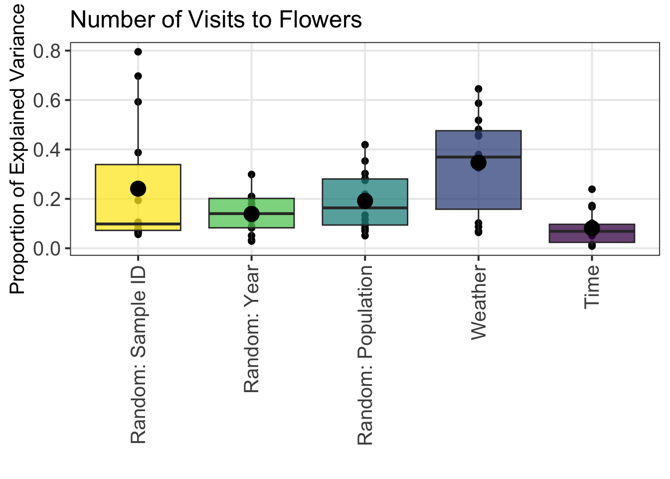
4.4.2 Specific Sources of Variance for Individual Pollinator Functional Groups
data_VP_model_time_weather_variance_partition %>%
  mutate(Source_Variance = factor(Source_Variance, levels = c("Random: Sample", "Random: Year", "Random: Population", "Weather", "Time_Start_Decimal"))) %>%
  ggplot(aes(x = Pollinator_Functional_Group, y = Variance_Proportion, fill = Source_Variance)) +
  geom_bar(position = "stack", stat = "identity", color = "black") +
  theme_bw(base_size = 15) +
  theme(legend.position = "right",
        legend.title = element_blank(),
        legend.text = element_text(size = 15),
        axis.text.x = element_text(angle = 90, vjust = 0.5, hjust = 1, size = 15),
        axis.text.y = element_text(size = 15),
        panel.grid.minor.y = element_blank()) +
  xlab("") +
  ylab("Proportion of Explained Variance") +
  scale_fill_manual(values = c("#FDE725", "#5DC963", "#21908D", "#3B528B", "#440154"),
                    labels = c("Random: Sample ID",
                               "Random: Year",
                               "Random: Population",
                               "Weather",
                               "Time")) +
  scale_x_discrete(labels=c(expression(italic("Bombus") ~ " Queen"),
                            expression(italic("Bombus") ~ " Worker"),
                            expression(italic("Bombus terrestris") ~ " Worker"),
                            "Bombyliidae",
                            "Coleoptera",
                            "Diurnal Lepidoptera",
                            "Honeybee",
                            "Large Solitary Bee",
                            "Noctuidae",
                            "Non-Syrphid Diptera",
                            "Other",
                            "Small Solitary Bee",
                            "Sphingidae",
                            "Syrphidae")) +
  ggtitle("Number of Visits to Flowers")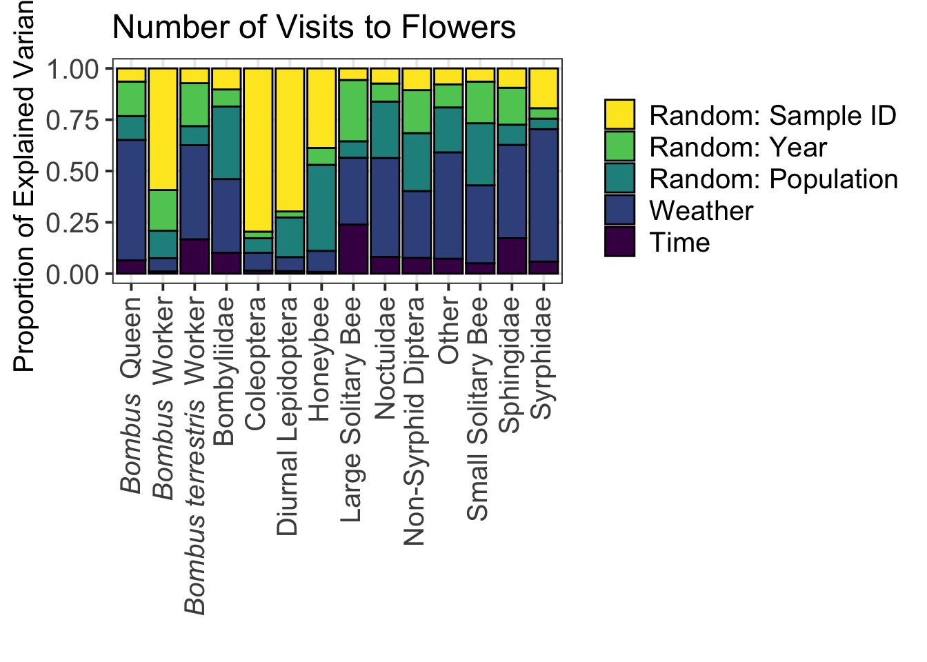
4.5 Questions Addressed By Variance Partitioning With HMSC
How much of the variation in species abundance is explained by spatial factors, temporal factors, and environmental factors?
What is the relative importance of spatial vs. temporal variation in explaining community structure?
Do different species exhibit similar spatial and temporal patterns of variation?
Are specific species more sensitive to particular environmental variables?
Which predictors explain the largest proportion of variance in community structure?