22 Day 22 (April 10)
22.1 Announcements
April check-in is worth 5% of your grade. Please send email to both Aidan and I to plan your April check in.
Selected questions/clarifications from journals
- Most questions are now project related.
- “I am currently struggling with the idea of what makes data”good” or “bad” and how that affects the design of a study.”
- “f you say you measured someone’s height, but the measurement method was poor or inconsistent, then the data may not be trustworthy at all….”
22.2 Gaussian process
- A Gaussian process is a probability distribution over functions
- If the function is observed at a finite number of points or “locations,” then the vector of values follows a multivariate normal distribution.
22.2.1 Multivariate normal distribution
Multivariate normal distribution
- \(\boldsymbol{\eta}\sim\text{N}(\mathbf{0},\sigma^{2}\mathbf{R})\)
- Definitions
- Correlation matrix – A positive semi-definite matrix whose elements are the correlation between observations
- Correlation function – A function that describes the correlation between observations
- Example correlation matrices
- Compound symmetry \[\mathbf{R}=\left[\begin{array}{cccccc} 1 & 1 & 0 & 0 & 0 & 0\\ 1 & 1 & 0 & 0 & 0 & 0\\ 0 & 0 & 1 & 1 & 0 & 0\\ 0 & 0 & 1 & 1 & 0 & 0\\ 0 & 0 & 0 & 0 & 1 & 1\\ 0 & 0 & 0 & 0 & 1 & 1 \end{array}\right]\]
- AR(1) \[\mathbf{R(\phi})=\left[\begin{array}{ccccc} 1 & \phi^{1} & \phi^{2} & \cdots & \phi^{n-1}\\ \phi^{1} & 1 & \phi^{1} & \cdots & \phi^{n-2}\\ \phi^{2} & \phi^{1} & 1 & \vdots & \phi^{n-3}\\ \vdots & \vdots & \vdots & \ddots & \ddots\\ \phi^{n-1} & \phi^{n-2} & \phi^{n-3} & \ddots & 1 \end{array}\right]\:\]
Example simulating from \(\boldsymbol{\eta}\sim\text{N}(\mathbf{0},\sigma^{2}\mathbf{R})\) in R
n <- 200
x <- 1:n
I <- diag(1, n)
sigma2 <- 1

library(MASS)
set.seed(2034)
eta <- mvrnorm(1, rep(0, n), sigma2 * I)
cor(eta[1:(n - 1)], eta[2:n])
## [1] -0.06408623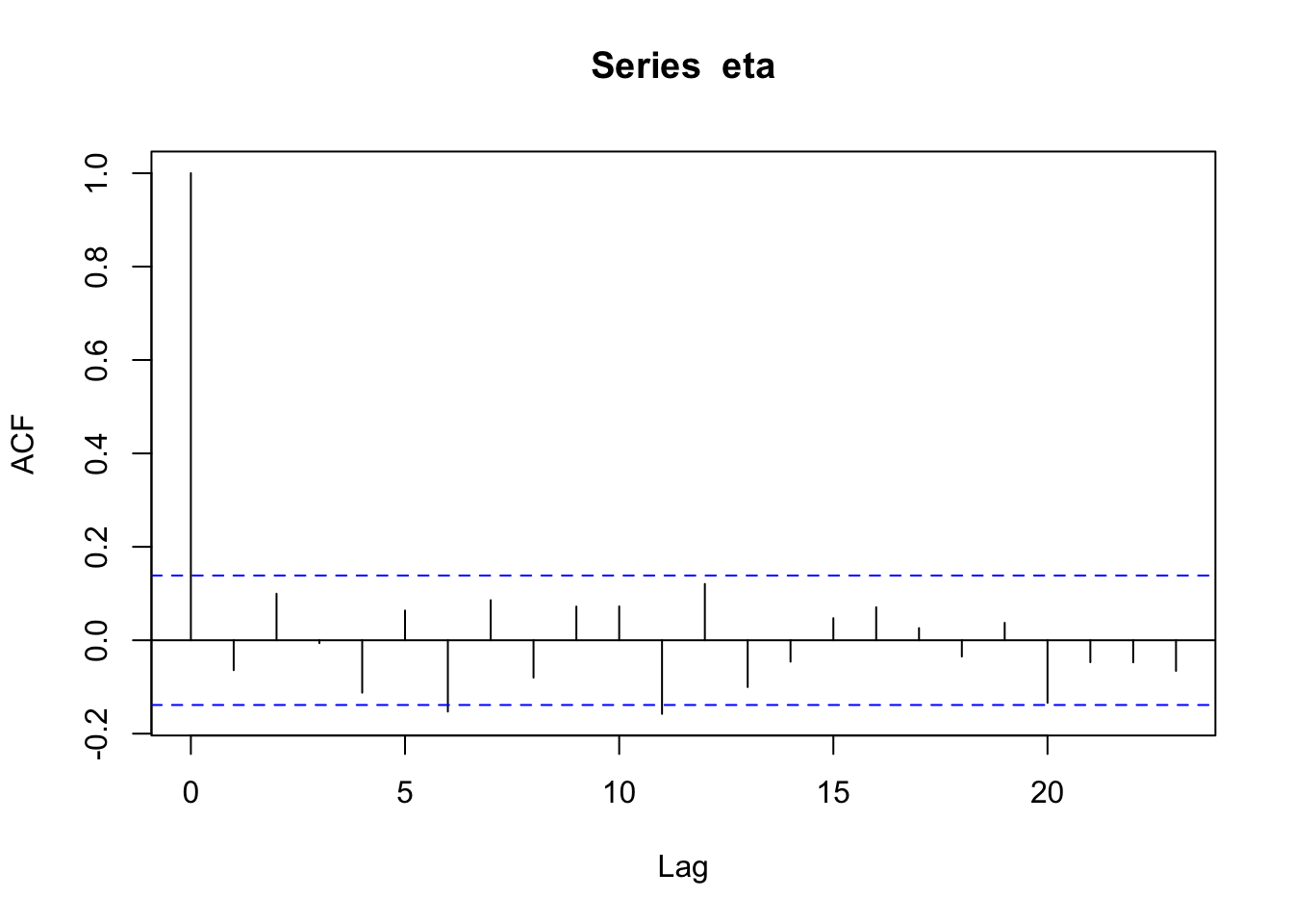
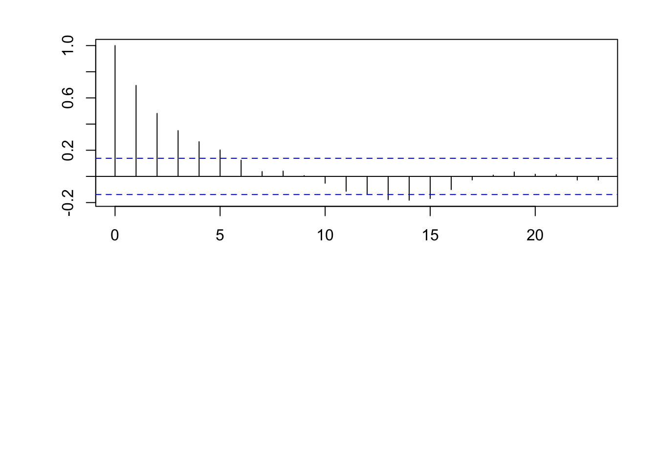
par(mfrow = c(2, 1))
par(mar = c(0, 2, 0, 0), oma = c(5.1, 3.1, 2.1, 2.1))
plot(x, eta, typ = "l", xlab = "", xaxt = "n")
abline(a = 0, b = 0)

n <- 200
x <- 1:n # Must be equally spaced
phi <- 0.7
R <- phi^abs(outer(x, x, "-"))
sigma2 <- 1
set.seed(1330)
eta <- mvrnorm(1, rep(0, n), sigma2 * R)
cor(eta[1:(n - 1)], eta[2:n])
## [1] 0.7016481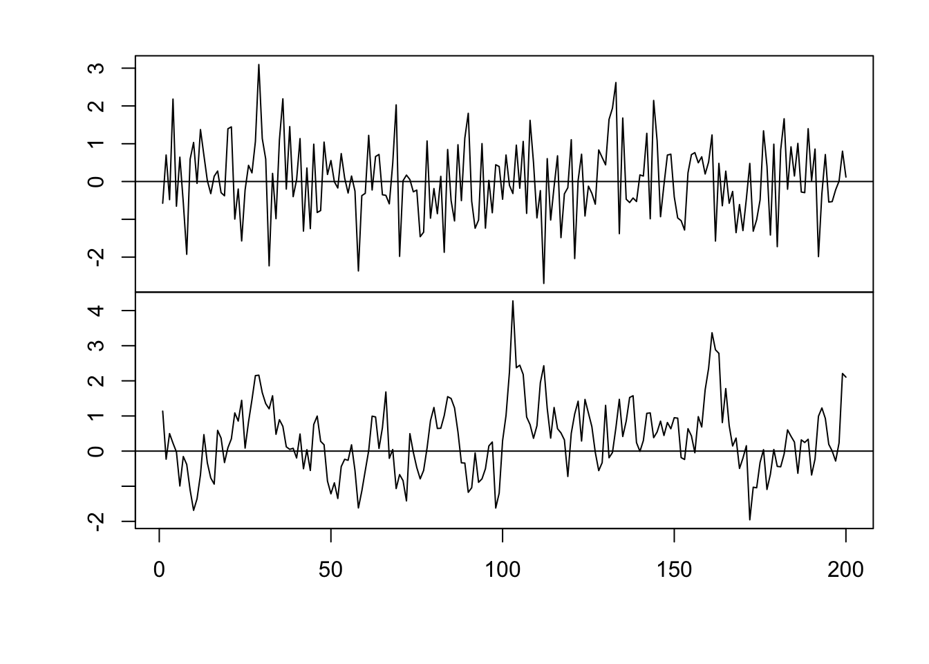
- Example correlation functions
- Gaussian correlation function \[r_{ij}(\phi)=e^{-\frac{d_{ij}^{2}}{\phi}}\] where \(d_{ij}\) is the “distance” between locations i and j (note that \(d_{ij}=0\) for \(i=j\)) and \(r_{ij}(\phi)\) is the element in the \(i^{\textrm{th}}\) row and \(j^{\textrm{th}}\) column of \(\mathbf{R}(\phi)\).
library(fields)
n <- 200
x <- 1:n
phi <- 40
d <- rdist(x)
R <- exp(-d^2/phi)
sigma2 <- 1

set.seed(4673)
eta <- mvrnorm(1, rep(0, n), sigma2 * R)
plot(x, eta, typ = "l")
abline(a = 0, b = 0)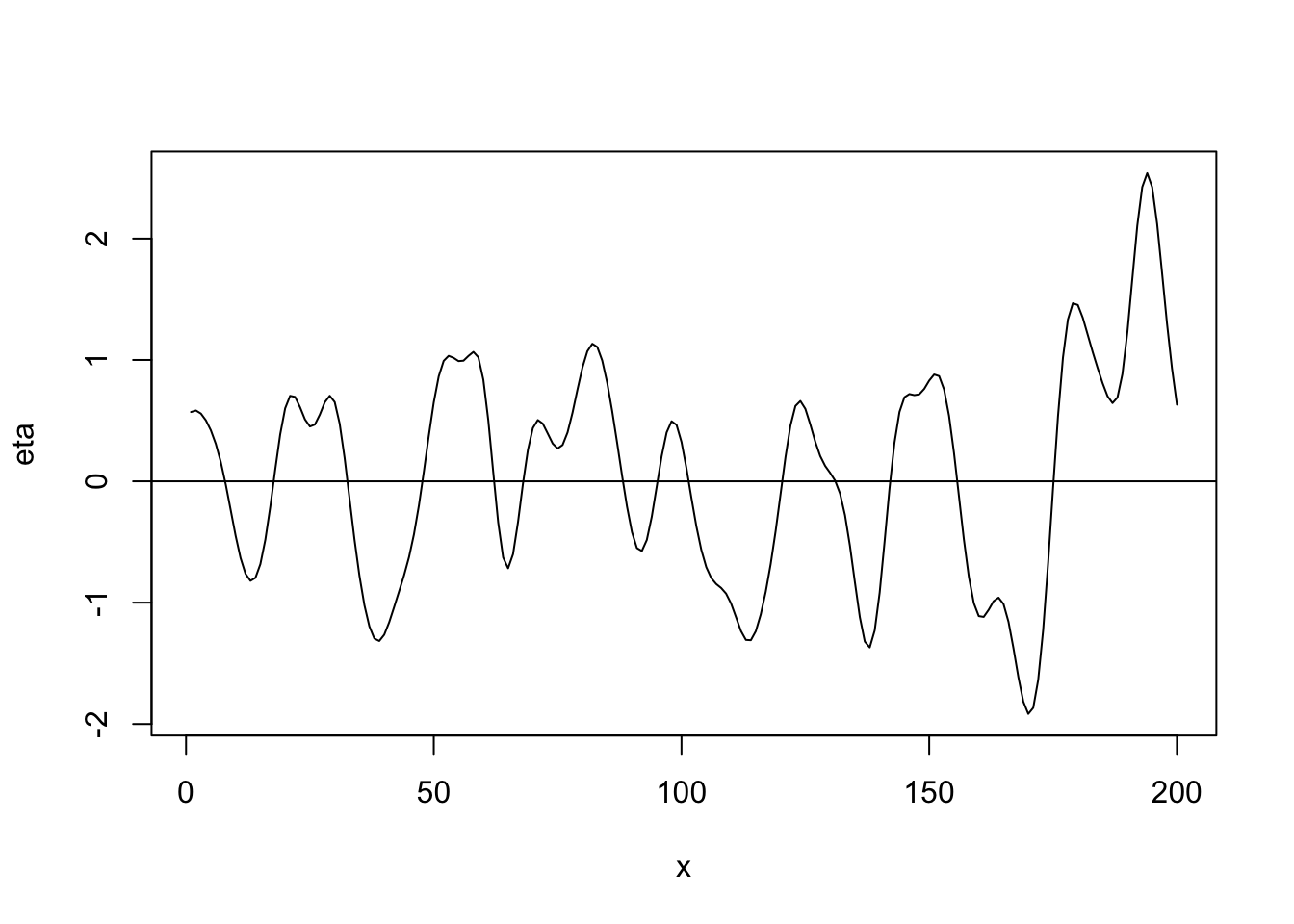
## [1] 0.9717508- Linear correlation function \[r_{ij}(\phi)=\begin{cases} 1-\frac{d_{ij}}{\phi} &\text{if}\ d_{ij}<0\\ 0 &\text{if}\ d_{ij}>0 \end{cases}\]
library(fields)
n <- 200
x <- 1:n
phi <- 40
d <- rdist(x)
R <- ifelse(d<phi,1-d/phi,0)
sigma2 <- 1

set.seed(4803)
eta <- mvrnorm(1, rep(0, n), sigma2 * R)
plot(x, eta, typ = "l")
abline(a = 0, b = 0)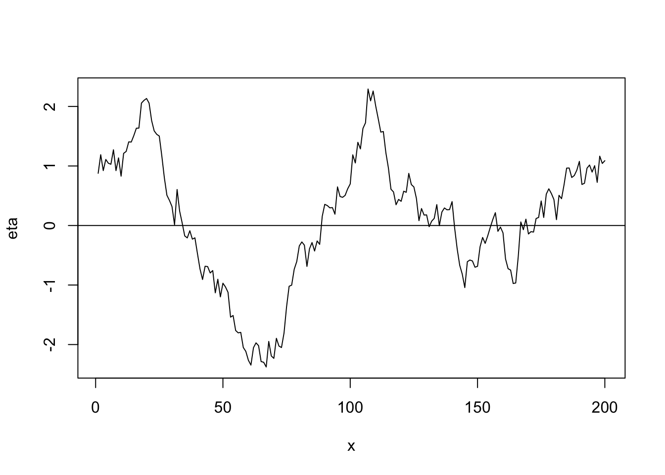
## [1] 0.9778878Bayesian Kriging
- Example correlation functions
Read Chapter 17
Example data set
url <- "https://www.dropbox.com/s/k2ajjvyxwvsbqgf/ISIT.txt?dl=1"
df <- read.table(url, header = TRUE)
df <- df[df$Station == 16,c(1,2,5,6)]

head(df)
## Depth Sources Latitude Longitude ## 595 598 53.37 49.0322 -16.1493 ## 596 631 51.32 49.0322 -16.1493 ## 597 700 42.42 49.0322 -16.1493 ## 598 666 38.32 49.0322 -16.1493 ## 599 1317 37.29 49.0322 -16.1493 ## 600 1352 36.27 49.0322 -16.1493plot(df$Depth, df$Sources, las = 1, ylim = c(0, 65), col = rgb(0, 0, 0, 0.25), pch = 19, xlab = "Depth (m)", ylab = "Sources")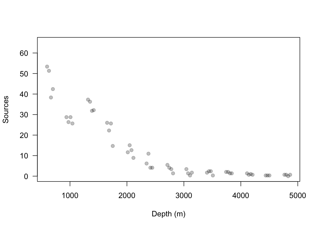
Modify the linear model
- Account for spatial autocorrelation
- Enable prediction at locations
- Write out on whiteboard
- In R
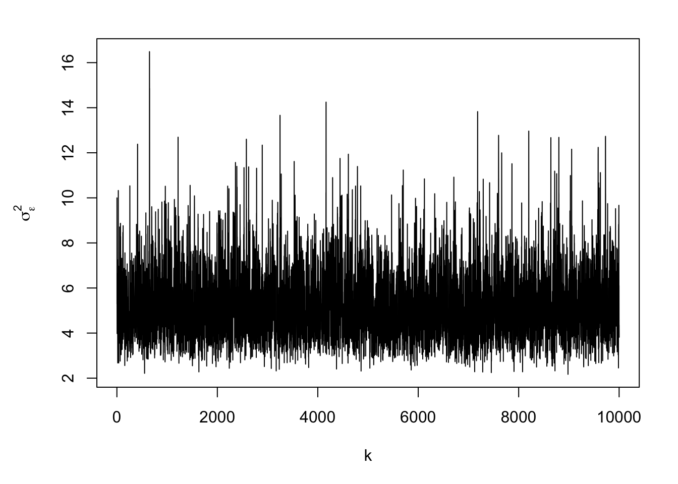
library(fields)
library(truncnorm)
library(mvtnorm)
library(coda)
library(MASS)

y <- df$Sources
X <- model.matrix(~I(Depth/Depth)-1,data=df)
Z <- diag(1,length(y))
n <- length(y)

# Distance matrix used to calculate correlation matrix
D <- rdist(df$Depth)

m.draws <- 10000  #Number of MCMC samples to draw
samples <- as.data.frame(matrix(,m.draws+1,dim(X)[2]+3))
colnames(samples) <- c(colnames(X),"sigma2.e","sigma2.alpha","phi")
samples[1,] <- c(40,10,150,250)  #Starting values for beta0, sigma2.e, sigma2.alpha, and phi
samples.alpha <- as.data.frame(matrix(,m.draws+1,length(y)))

# Hyperparameters for priors
sigma2.beta <- 100
a <- 2.01
b <- 1
c <- 2.01
d <- 1
e <- 0
f <- 10^6

accept <- matrix(, m.draws + 1, 1) # Monitor acceptance rate
colnames(accept) <- c("phi")
phi.tune <- 10

set.seed(3909)
ptm <- proc.time()
for(k in 1:m.draws){
  beta <- t(samples[k,1:dim(X)[2]])
  sigma2.e <- samples[k,dim(X)[2]+1]
  sigma2.alpha <- samples[k,dim(X)[2]+2]
  phi <- samples[k,dim(X)[2]+3]
  C <- exp(-(D/phi)^2)
  CI <- solve(C)

  # Sample alpha
  H <- solve((1/sigma2.e)*t(Z)%*%Z + (1/sigma2.alpha)*CI)
  h <- (1/sigma2.e)*t(Z)%*%(y-X%*%beta)
  alpha <-  mvrnorm(1,H%*%h,H)

  # Sample beta
  H <- solve((1/sigma2.e)*t(X)%*%X + (1/sigma2.beta)*diag(1,dim(X)[2]))
  h <- (1/sigma2.e)*t(X)%*%(y-Z%*%alpha)
  beta <-  mvrnorm(1,H%*%h,H)

  # Sample sigma2.alpha
  sigma2.alpha <- 1/rgamma(1,a+n/2,b+t(alpha)%*%CI%*%(alpha)/2)

  # Sample sigma2.e
  sigma2.e <- 1/rgamma(1,c+n/2,d+t(y-X%*%beta-Z%*%alpha)%*%(y-X%*%beta-Z%*%alpha)/2)

  #Sample phi
  phi.star <- rnorm(1,phi,phi.tune)
  if(phi.star > e & phi.star < f){
C.star <-  exp(-(D/phi.star)^2)
mh1 <- dmvnorm(alpha,rep(0,n),sigma2.alpha*C.star,log=TRUE) + dunif(phi.star,e,f,log=TRUE)
mh2 <- dmvnorm(alpha,rep(0,n),sigma2.alpha*C,log=TRUE) + dunif(phi,e,f,log=TRUE)
R <- min(1,exp(mh1 - mh2))
if (R > runif(1)){phi <- phi.star}}

  # Save
  samples[k+1,] <- c(beta,sigma2.e,sigma2.alpha,phi)
  samples.alpha[k+1,] <- alpha
  accept[k+1,] <- ifelse(phi==phi.star,1,0)
  if(k%%1000==0) print(k)
}
## [1] 1000 ## [1] 2000 ## [1] 3000 ## [1] 4000 ## [1] 5000 ## [1] 6000 ## [1] 7000 ## [1] 8000 ## [1] 9000 ## [1] 10000## user system elapsed ## 18.591 1.490 20.114## [1] 0.3744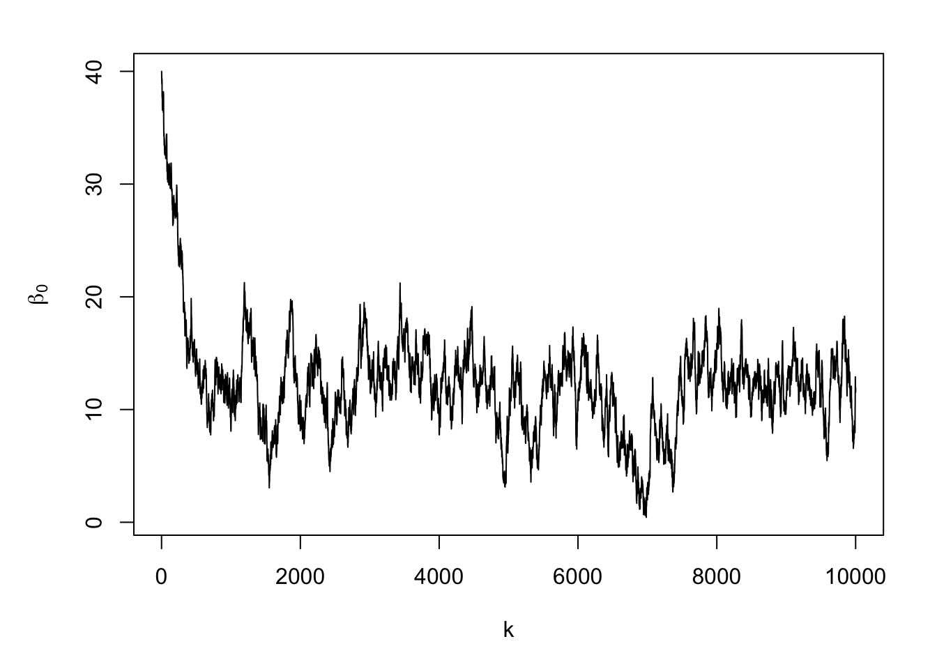
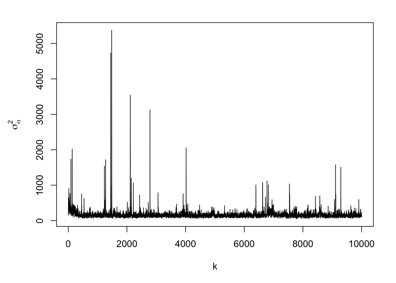
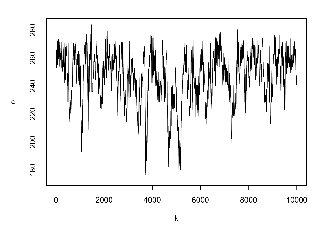
#Note: there is a trace plots for each of the 51 alphas
plot(samples.alpha[,1],typ="l",xlab="k",ylab=expression(alpha))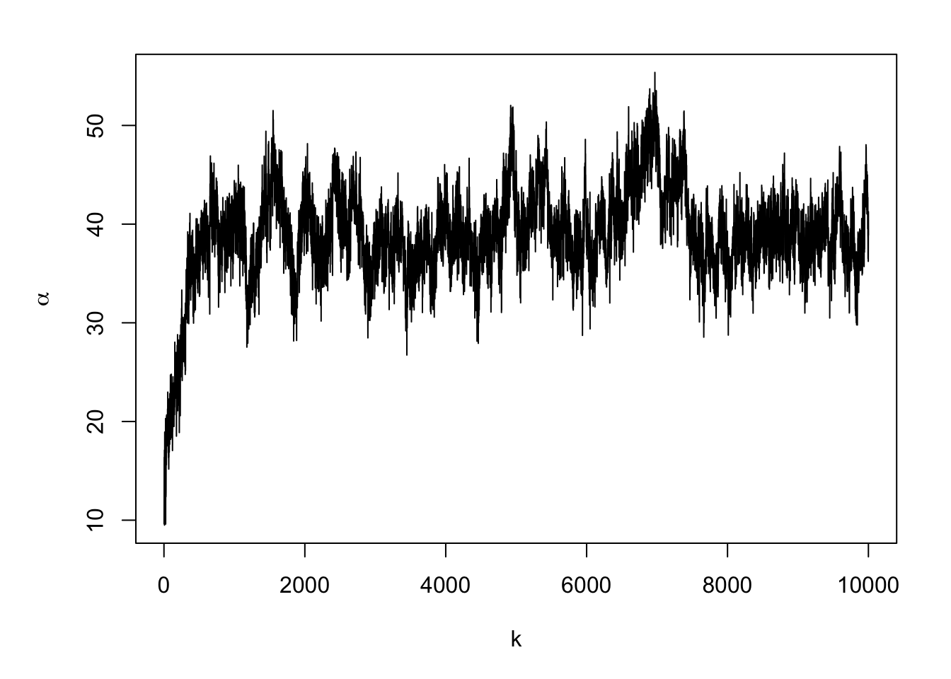
## I(Depth/Depth) sigma2.e sigma2.alpha phi ## 39.51309 3283.46774 965.35201 58.74402## V1 V2 V3 V4 V5 V6 V7 V8 ## 59.56160 49.82792 57.07751 48.99081 53.30777 43.70968 55.38660 45.69857 ## V9 V10 V11 V12 V13 V14 V15 V16 ## 49.93532 47.14301 44.15401 53.99566 54.05355 45.99079 47.52021 45.34204 ## V17 V18 V19 V20 V21 V22 V23 V24 ## 53.59280 49.23023 52.45801 46.94143 56.66246 53.20491 51.57685 47.47904 ## V25 V26 V27 V28 V29 V30 V31 V32 ## 55.16787 47.17939 47.32656 50.79651 45.51036 48.02659 54.54050 47.49616 ## V33 V34 V35 V36 V37 V38 V39 V40 ## 50.32102 53.67834 53.26875 45.94377 46.86828 54.00938 55.75524 48.21335 ## V41 V42 V43 V44 V45 V46 V47 V48 ## 50.72585 53.72889 51.05043 47.42698 57.13272 43.55410 51.78176 52.50197 ## V49 V50 V51 ## 48.57829 51.98884 49.18213## I(Depth/Depth) sigma2.e sigma2.alpha phi ## 11.603376 5.129544 163.061302 245.726972## I(Depth/Depth) sigma2.e sigma2.alpha phi ## 2.5% 3.810371 3.003591 80.09624 201.3898 ## 97.5% 17.776531 8.592822 335.24769 270.9082# obtain E(y) of at new depths new.depth <- seq(min(df$Depth),max(df$Depth),by=10) X.new <- model.matrix(~I(new.depth/new.depth)-1) Z.new <- diag(1,length(new.depth)) D.cross <- rdist(new.depth,df$Depth) samples.pred <- matrix(,length(burn.in:m.draws),length(new.depth)) for(k in burn.in:m.draws){ alpha <- t(samples.alpha[k,]) beta <- t(samples[k,1:dim(X)[2]]) sigma2.e <- samples[k,dim(X)[2]+1] sigma2.alpha <- samples[k,dim(X)[2]+2] phi <- samples[k,dim(X)[2]+3] C <- exp(-(D/phi)^2) C.cross <- exp(-(D.cross/phi)^2) alpha.new <- C.cross%*%solve(C)%*%alpha samples.pred[k-burn.in+1,] <- X.new%*%beta + Z.new%*%alpha.new } plot(df$Depth,df$Sources,las=1,ylim=c(0,60),col=rgb(0,0,0,0.25),pch=19, xlab="Depth (m)",ylab="Sources") points(new.depth,colMeans(samples.pred),typ="l")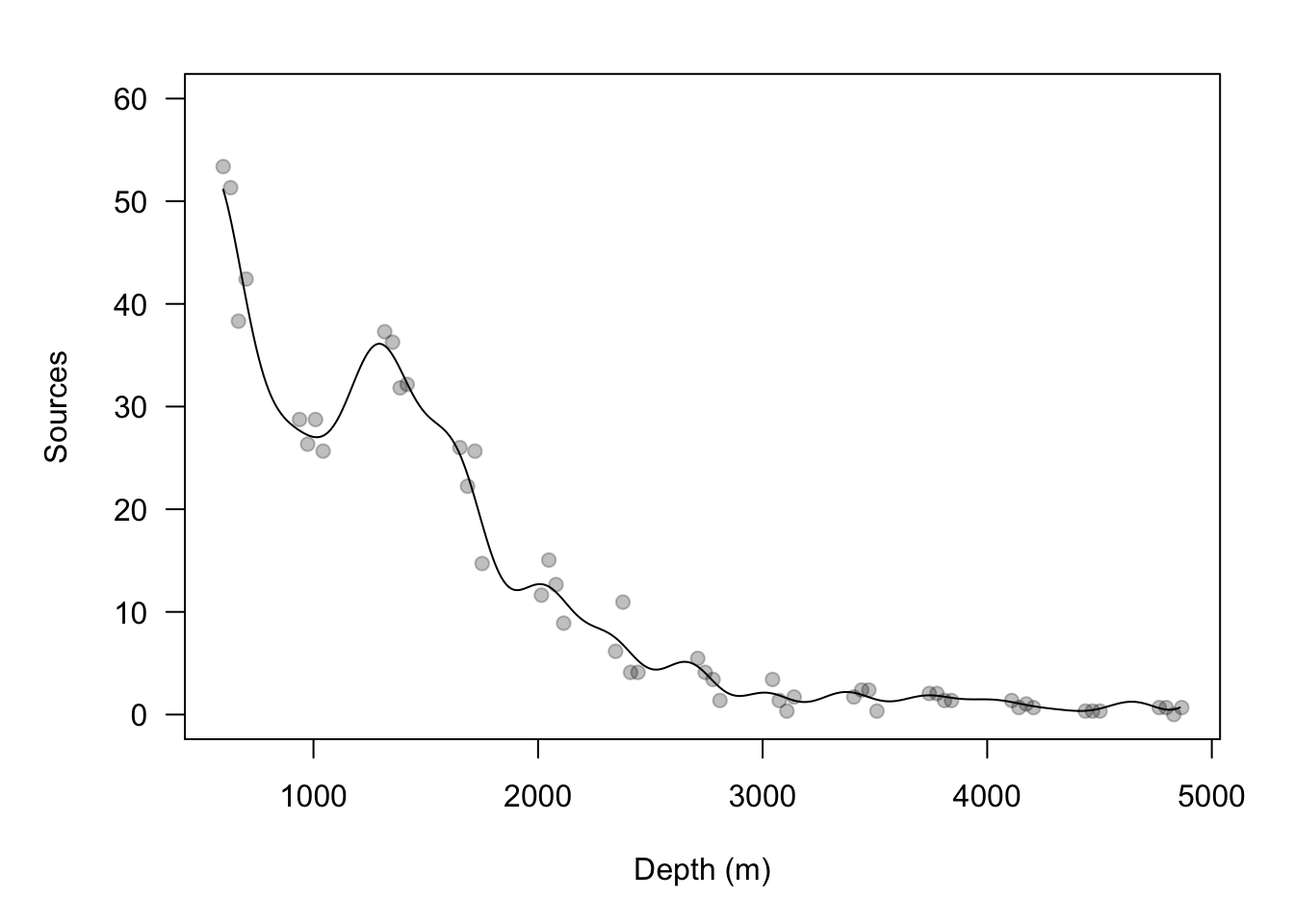
EV.beta <- mean(samples[-c(1:burn.in),1])
EV.alpha <- colMeans(samples.alpha[-c(1:burn.in),])
EV.e <- y - X%*%EV.beta - Z%*%EV.alpha

par(mfrow=c(2,1))
plot(df$Depth, EV.e, las = 1, col = rgb(0, 0, 0, 0.25),pch = 19, xlab = "Depth (m)", ylab = expression("E("*epsilon*")"))
hist(EV.e,col="grey",main="",breaks=10,xlab= expression("E("*epsilon*")"))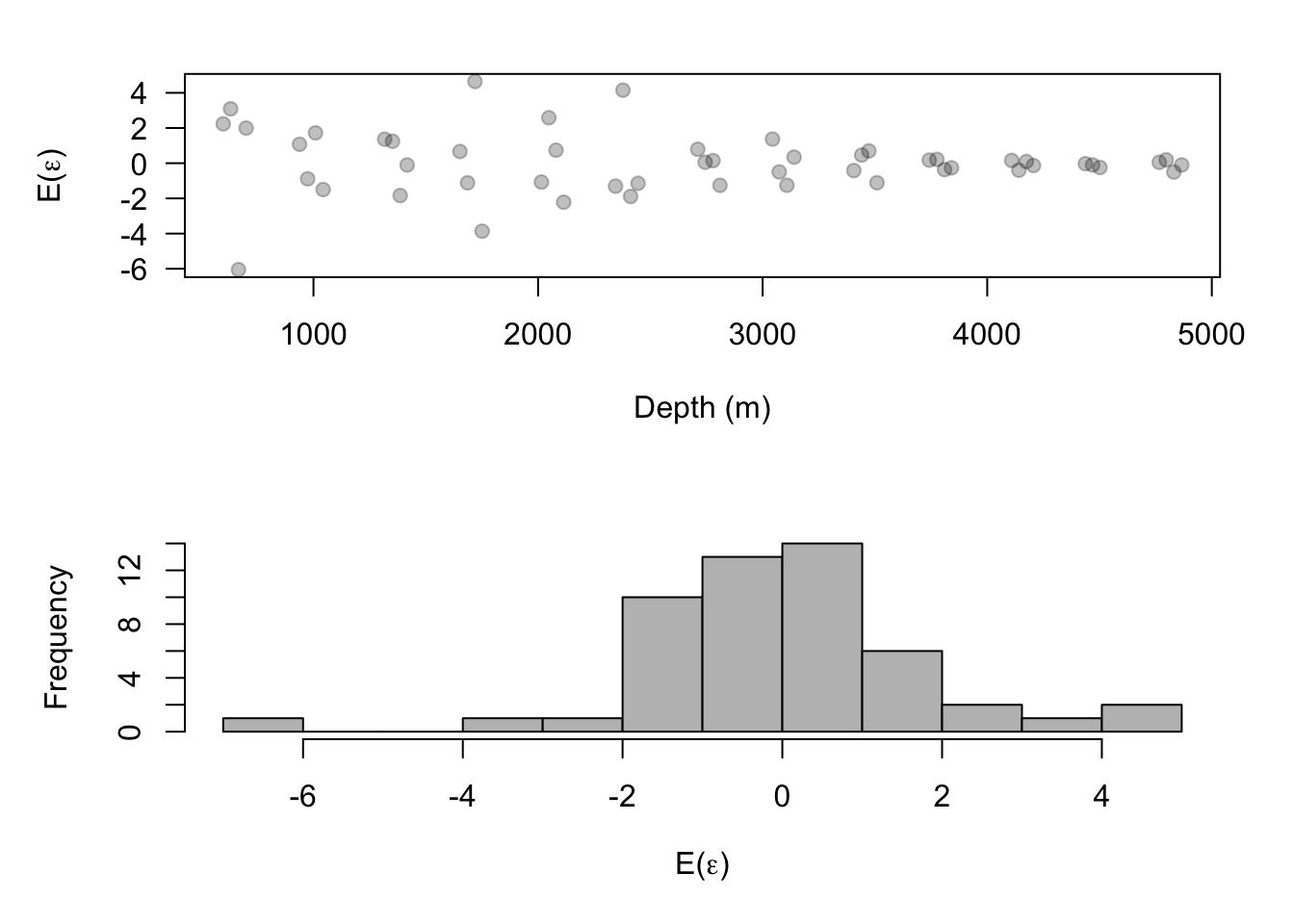
22.3 Extreme precipitation in Kansas
- On September 3, 2018 there was an extreme precipitation event that resulted in flooding in Manhattan, KS and the surrounding areas. If you would like to know more about this, check out this link and this video.
- Live example (Download here[https://drive.google.com/file/d/1JKOf3HRZ8Mry0MrHSLfWVPL-KmG6IeeC/view?usp=sharing])