1.2 Recalling of R programming environment

R is open-source software, meaning it is free to use, modify, and distribute. It enables quick upgrading and continuous development of new methods and models for econometric analysis (unlike alternative softwares which are not free).
It’s main advantage is that intuitive code (commands) can be easily extended and/or customized to meet user needs
You can easily copy existing commands and replicate the same examples at home. Complex analyses can be automated and reproduced on a new data.
It is available for Windows, Mac, and Linux platforms
With the first installation, you get base packages that support commands for basic statistical and graphical data analysis
Along with R, it is recommended to install RStudio, an integrated development environment (IDE) that simplifies the coding process and makes it easier to work with R, as includes many useful features such as an interactive console, visualization tools, script editor, workspace environment, packages library, command history, etc.
Two steps installation on your PC -> first R and then RStudio

First step installation requires a choice of Comprehensive R Archive Network (CRAN) repository through which additional packages, for some “advanced” analysis, are available. Latter, you should click Download R for Windows and select install R for the first time (latest version)
Second step installation requires downloading and installing RStudio Desktop
There is also a cloud version of RStudio called Posit Cloud, which allows users to run RStudio in a web browser without needing to install anything locally
In \(2022\), RStudio rebranded as Posit, reflecting its expansion and integration with Python
RStudio cloud version is also free and available on this link https://posit.cloud/
The easiest way to access Posit Cloud is to log in with Google account (even if you are a first time user)
After running RStudio (on your PC or web browser) the user interface will look similar to the next screen

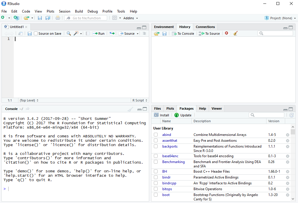
FIGURE 1.1: RStudio user interface

Unnamed file in the upper right corner Untitled1 is newly opened and empty R Script in which you write commands by hand (File -> New File -> R Script)
Arguments for each command are written inside parentheses ( )
Command is computed by selecting it with the mouse and clicking the Run button or by using the shortcut Ctrl+Enter at the end of the command line
It is useful to write a comments (lines beginning with #) which are ignored by R. Comments are useful for making short notes in explaining your codes.
In the lower left corner a Console window prints the results as well as warnings and errors (for example, the syntax of the command is incorrectly written or the specific command/object is not found)
Right side window panes serve to track the steps of the analysis, including History, Plots, Help, Packages (shows the list of currently installed packages in the library), etc.
Save the R script with an arbitrary name of your choice if necessary (File -> Save as \(\dots\))
You can load a saved script into RStudio at any time, and the commands in that script will be recomputed by selecting them again and clicking the Run button
According to the RStudio settings, all scripts (with extension .R) are saved in your working directory; usually My Documents or Desktop

getwd() # Information about your current working directory
setwd("new path") # Working directory can be changed by setting a new path

R can be used as calculator, data in R can be simulated by some random number generator (RNG) or imputed by hand
in R data can be also imported from locally saved files or if the data file is available online it can be loaded directly into RStudio using URL link address
If a CSV file is available online (comma-separated values), you should use read.csv() command instead of read.table()
To import Excel files, it is recommended to use read_excel() command from the readxl package
Furthermore, data can be directly loaded into RStudio from public sources. Several packages support commands for direct loading of secondary data.

To load data from EUROSTAT, you should first check the data navigation tree at https://ec.europa.eu/eurostat/data/database to locate and identify the dataset code of interest, as well as the country codes, variable/indicator codes, and other relevant filters
Knowing specific commands in RStudio for working with vectors and matrices is extremely useful for data manipulation, including transforming, reshaping, and aggregating the data

TABLE 1.3: Working with vectors
Command	Description
`c(a,b,c,d,...)`	vector with elements \(a\), \(b\), \(c\), \(d\), …
`seq(n)`	sequence from \(1\) to \(n\)
`seq(a:n)`	sequence from \(a\) to \(n\)
`seq(a,n,c)`	sequence from \(a\) to \(n\) in steps \(c\)
`rep(a,n)`	vector with \(n\) equal elements \(a\)
`length(v)`	number of elements in vector \(v\)
`sum(v)`	sum of the elements of vector \(v\)
`prod(v)`	product of the elements of vector \(v\)

TABLE 1.4: Working with matrices
Command	Description
`matrix(v, nrow=n)`	matrix with elements of \(v\) in \(n\) rows
`cbind(c1, c2, ...)`	combines more columns into a matrix
`rbind(r1, r2, ...)`	combines more rows into a matrix
`diag(A)`	extracts diagonal elements of a matrix \(A\)
`diag(n)`	creates identity matrix with dimensions \(n \times n\)
`t(A)`	transposes matrix \(A\)
`solve(A)`	inverse of a matrix \(A\)
`A %*% B`	multiplication of two matrices \(A\) and \(B\)
`dim(A)`	dimensions of a matrix \(A\)

Along with data frames, vectors, and matrices, you can work with other types of objects in R, such as arrays, lists or time-series objects (xts or zoo). While a matrix is similar to a data frame, it does not have column names or row names.
Each column in a data frame is a vector of the same length, but unlike a matrix, the columns of a data frame can hold different data types. In contrast, all columns in a matrix must be numeric.