Chapter 8 Modeling with ODEs
In this section we investigate a key area of interest for ordinary differential equations – modeling. ODEs are often used to model physical phenomena as they allow us to express a relationship between an unknown quantity, \(y\), and the rate of change of the unknown quantity \(y'\). In this section we will model with autonomous ODEs. Many physical and biological phenomena can be modeled using autonomous ODE, and the special structure of autonomous ODEs allow us to extract certain types of solutions, called equilibrium solutions, with little effort.
8.1 Exponential Models
8.1.1 Exponential Population Growth
Consider a population of bacteria living a Petri dish. Let \(P(t)\) be the population of bacteria in the dish at time \(t\). Assume that \(t\) is measured in hours. When using differential equations to model a physical phenomenon, we often begin by asking if we can express the rate of change of the quantity in a simple way. That is, we are looking for an expression for \(P'(t)\).
One of the most common models for modeling a population is to assume that the rate of change on the population is proportional to the current population. In this context, this means that if there are only two bacteria present at time \(t\), the population can’t be growing too quickly, since there are only bacteria present to divide. However, if there are 1000 bacteria present, then there are many cells present to divide, and so will be quickly adding new bacteria to the population.
If the rate of change of the population, \(P'(t)\) is proportional to the current population, \(P(t)\), then we have \[P'(t)=kP(t)\] where \(k\) is a growth parameter. If \(k\) is a large number, the population grows quickly. If \(k\) is a small, positive, number, then the population grows slowly. If \(k\) is a negative number, then the population decreases, since then we would have \(P'(t)<0\). The dimension of \(k\) is \(1/T\). This means that the dimension \(1/k\) is \(T\). It turns out that \(1/k\) is the average amount of time a cell spends “resting” between divisions.
8.1.1.1 Example
Suppose that a bacterial colony initially has 100 members, that the rate of change of the population is proportional to the current population, and that on average a cell spends 5 hours resting between cell divisions. Find a formula for the population of the colony at time \(t\).
Let \(P(t)\) be the population at time \(t\), where \(t\) is in hours. Since the rate of change of the population is proportional to the current population, \[P'=kP.\] Since the average amount of time between cell divisions is \(\frac{1}{k}=5\) hours, we have \(k=\frac{1}{5}\) hour\(^{-1}\). We have \[P'=\frac{1}{5}P.\] This equation is separable. Our standard method for solving separable differential equations (assuming \(P>0\)) gives us an answer. \[\begin{aligned} &\frac{dP}{dt}=\frac15 P\\ &\frac{1}{P}\frac{dP}{dt}=\frac{1}{5}\\ &\int \frac{1}{P}\frac{dP}{dt} dt = \int \frac15 dt\\ &\int \frac{1}{P}dP = \int \frac15 dt\\ &\ln(P) = \frac{1}{5} t + C_1\\ &P=e^{1/5 t+C_1} = Ce^{1/5 t}. \end{aligned} \]
We can use our initial condition to determine \(C\). \[100=P(0)=Ce^{1/5\cdot 0} = C.\] Finally, we have our specific solution to the IVP. \[P=100e^{1/5 t}.\] You might recall this function from Block 1. This model is called exponential growth. As we saw in Block 1, \(\ln(2)/k\) is the doubling time of the population.
Here we can see a strength of differential equations. The model \(P=Ce^{kt}\) is difficult to interpret. When modeling a population, it is not clear that the model should be exponential, rather than , e.g., a power function or any other function that grows quickly. It is not clear that the growth rate should appear in the power rather than as a coefficient. However, the model \(P'=kP\) is easy to interpret and as expressing an assumption that we think is reasonable, that the rate of growth of a population is proportional to the population itself. The formula \(P=Ce^{kt}\) comes about as a consequence of this believable assumption.
8.1.2 Radioactive Decay
Another example of modeling with a 1\(^{st}\) order, autonomous ODE is the decay of a radioactive element. Atoms that are radioactive spontaneously decay into atoms of a different element. Let \(y(t)\) be the mass of our radioactive element present at time t.
The most common assumption regarding the rate of change of \(y\) is that the rate of change of the amount of element present is proportional to the amount of the element present. Where there are many atoms of our radioactive element present, there are many atoms available to transmute, and thus we can lose a lot of radioactive substance quickly. When there is little of our element present, there are few atoms available to transmute, so we can’t lose material quickly.
As with population growth, if the rate of change of the amount present is proportional to the amount present, then \[\frac{dy}{dt} = k y.\] If we expect the amount of isotope present to decay, then we expect that \(k<0\), so that \(\frac{dy}{dt}<0\). The more negative (large but negative) \(k\) is, the faster the isotope decays.
As with population models, the dimension of \(k\) is time\(^{-1}\). Therefore \(\frac{1}{k}\) has dimension time. While the quantity \(1/k\) is more difficult to interpret than in population models, it is true that the quantity \(\frac{-\ln(2)}{k}\) has dimension time and can be interpreted as the halving time, or half-life, of the element. That is, \(\frac{-\ln(2)}{k}\) tells us how long it will take for one half of our current mass of element to radiate away.
8.1.2.1 Example
Francium-223 (Fr-223) has a half-life of roughly 22 minutes. Assume that at time 0 we have a stockpile of 50 kg of francium-223.
- Build a differential equation model for \(y(t)\), the amount, in kg, of francium 223 present at time \(t\).
- Solve the differential equation model for \(y(t)\).
- Determine how much francium-223 will be present after 30 minutes of decay.
- Determine how long it will take for exactly 15 kg of francium-223 to remain.
Solution
Assuming that the rate at which Fr-223 (in kg/min) is proportional to the amount of Fr-223 present (in kg), which is a reasonable model for radioactive decay, then \[y'=ky.\] The constant \(k\) is related to the half-life by \[\frac{-\ln(2)}{k} \text{ min } = 22 \text{ min }.\] Therefore,
\[k=\frac{-\ln(2)}{22}\approx -0.032 \text{ min}^{-1}.\]
Our IVP is therefore \[y'=-0.032 y,\quad y(0)=50.\]
As with the population model, the solution to this IVP is
\[y=50e^{-0.032t}.\]
The amount present after 30 minutes will be
\[y(30)=50e^{-0.032 \cdot 30}\approx 19.145 \text{ kg}.\]
In order to find a time \(t\) at which there are 15 kg of Fr-223 to remain, we need to solve
\[15=50 e^{-0.032 t}\]
for \(t\).
\[\begin{aligned}
&\frac{15}{50}= e^{-0.032 t}\\
&\ln\left(\frac{15}{50}\right)=-0.032 t\\
&\frac{1}{-0.032}\ln\left(\frac{15}{50}\right)=t\\
&t\approx 37.624.\end{aligned}
\]
Alternatively, we can use findZeros to solve
\[50e^{-0.032t}-15=0.\]
##        t
## 1 37.624
8.1.3 Continuously Compounded Interest
Many types of financial accounts accrue interest on deposits. Interest is sometimes compounded annually, quarterly, weekly, or daily. When the compounding is very frequent,like daily, it becomes convenient to imagine that the compounding is done continuously. That is, we imagine that at all times the balance of the account is growing due to interest accumulation.
The amount of interest the account generates is directly proportional to the amount of principle in the account. A differential equation modeling the balance of the account at time \(t\), \(P(t)\), is \[P'=rP.\] Here, the coefficient \(r\) is the annual interest rate if \(t\) is measured in years, which is by far the most common situation.
We can see that this is another exponential growth model, as in Section 8.1.1 the solution to this problem is \[P=P_0 e^{rt},\] where \(P_0\) is the initial principle deposited in the account.
A more interesting situation is when money is deposited or withdrawn to/from the account. If the money is deposited frequently, for instance at the end of every business day, it is convenient tot think of the money being added to the account continuously. If the money is added/withdrawn at constant rate \(I\) (money per time) then a differential equation describing the situation is \[P'=rP+I.\]
8.1.3.1 Example
Consider a bank account with an annual interest rate of 3.5%. Your current account balance is a respectable $13,000. Rather than compounding monthly, the bank compounds interest daily, so that we might consider the compounding continuous. Your employer offers you a bonus, but offers you a choice. You can either have $5000 deposited in your account dispersed evenly over the year (an equal amount deposited every business day into your account), or you can have $5100 deposited in your account at the end of the year. Which should you take?
Solution
First we consider the outcome of a lump sum payment. Because we won’t be adding money to the account other than the continuously compounded interest, the value of the account at time \(t\) will solve the IVP \[P'=0.035P,\quad P(0)=13000.\] The solution to this IVP is \[P=13000e^{0.035t}.\] Since time is measured in years, the value of the account after one year is \[P(1)=13000e^{0.035\cdot 1}\approx 13463.06.\] Adding on the $5100 bonus at the end of the year, we get a total account value of $18563.06.
If we take the money at the continuous rate of $5000 per year, as our employer suggests, the IVP describing our account value is \[P'=0.035P + 5000,\quad P(0)=13000.\] This is an autonomous differential equation that we can solve using separation of variables.
\[\begin{aligned} &\frac{dP}{dt}=0.035P+5000\\ &\frac{1}{0.035P+5000}\frac{dP}{dt}=1\\ &\int \frac{1}{0.035P+5000}\frac{dP}{dt}\,dt=\int 1\,dt\\ &\int \frac{1}{0.035P+5000}dP=\int 1\,dt\\ &\frac{1}{0.035}\ln\left(0.035P+5000\right)=t+C_1\\ &\ln\left(0.035P+5000\right)=0.035t+0.035C_1\\ &0.035P+5000=e^{0.035t+0.035C_1}\\ &0.035P=e^{0.035t+0.035C_1}-5000\\ &P=\frac{1}{0.035}e^{0.035t+0.035C_1}-\frac{5000}{0.035}\\ &P=\frac{1}{0.035}e^{0.035t}e^{0.035C_1}-142857.1\\ &P=Ce^{0.035t}-142857.1\\ \end{aligned}\] Using the initial condition \(P(0)=13000\) we get \[\begin{aligned} &13000 = P(0) = Ce^{0.035\cdot 0}-142857.1 = C-142857.1\\ &C=13000 + 142857.1 \approx 155857.1. \end{aligned}\] Therefore \(P(t) = 155857.1e^{0.035t}-142857.1\). Finally, the value of the account after one year is \[P(1)=155857.1e^{0.035\cdot 1}-142857.1 \approx 18551.59.\] Using the continuous compounding of our money throughout the year, our account now has value $18551.59, compared to $18563.06 if we take the lump sum bonus at the end of the year. Thus, the larger bonus is still preferable, in this case, though it is much closer than one might suspect.
Note that rather than solving these differential equations analytically, we could use Euler with a very small step size. We should use a small step size because Euler’s method is an approximation, and small step sizes help us ensure accuracy. Notice that the results of Euler’s method at time \(t=1\) year are still off by a penny. On the other hand, using Euler’s method saves us much algebra!
##          t        P
## 999  0.998 13462.11
## 1000 0.999 13462.58
## 1001 1.000 13463.05## t P
## 999 0.998 18540.19
## 1000 0.999 18545.84
## 1001 1.000 18551.498.2 Logistic Equation
As we saw in Block 1 of this course, exponential models predict that the population in question will grow forever. This, of course, is unrealistic. In Block 1 of this course we updated our models to level off after some time; mathematically this meant moving from exponential models to sigmoidal models.
Exponential models come from the simple differential equation \[\frac{dP}{dt}=kP.\] Sigmoidal models come from the more involved logistic differential equation, commonly called the logistic equation. \[\frac{dP}{dt}=kP\left(1-\frac{P}{M}\right).\] The logistic equation comes from two observations.
First, when the population is small, the population should grow exponentially. This is reflected mathematically because when \(P\) is much smaller than \(M\), \(P/M\) is very nearly 0, and so \(\frac{dP}{dt}\approx kP\). So the logistic equation predicts nearly exponential growth when the population is small. Indeed, the parameter \(k>0\) is still a growth rate with dimension time\(^{-1}\).
Second, there is a population, called the carrying capacity, past which the population cannot grow. In the logistic equation, the carrying capacity is the parameter \(M\). \(M\) has dimension of population. We can see that if, somehow, the population ever becomes larger than \(M\) then \(P/M\)>1, and so \(\frac{dP}{dt}<0\). That is, if the population ever becomes larger than \(M\), the population will decrease.
There are a variety of equations that would satisfy our two criteria above, but the logistic equation is the simplest. The logistic equation can be solved by hand; however, we will not do so in this course. Instead, we can use our numerical methods to answer any questions we might have.
8.2.0.1 Example
Consider a population of squirrels, \(S(t)\). When the population of squirrels is small and resources are not an issue, the rate at which squirrels reproduce is proportional to their population, with a growth rate \(k = 0.3\) week\(^{-1}\). However, the squirrels live in a park with enough food and space to support a maximum population of 225 squirrels. At time 0, we have observed that 10 squirrels live in the park.
- Write an IVP to model this situation.
- Use
plotODEDirectionFieldto draw a direction field for the ODE. - Using the direction field, determine the long-term population of the squirrels int the park.
- Use
Eulerto predict the population of squirrels after 5 weeks. - Use
Eulerto predict the time at which the population will reach 150 squirrels.
Solution
We are given that the growth rate is \(k=0.3\) week\(^{-1}\), and that the carrying capacity of the park is \(M=225\). The initial population is \(S(0)=10\). The IVP corresponding to the situation is \[\frac{dS}{dt}=0.3S\left(1-\frac{S}{225}\right),\quad S(0)=10.\] We can plot a direction field for this autonomous ODE.
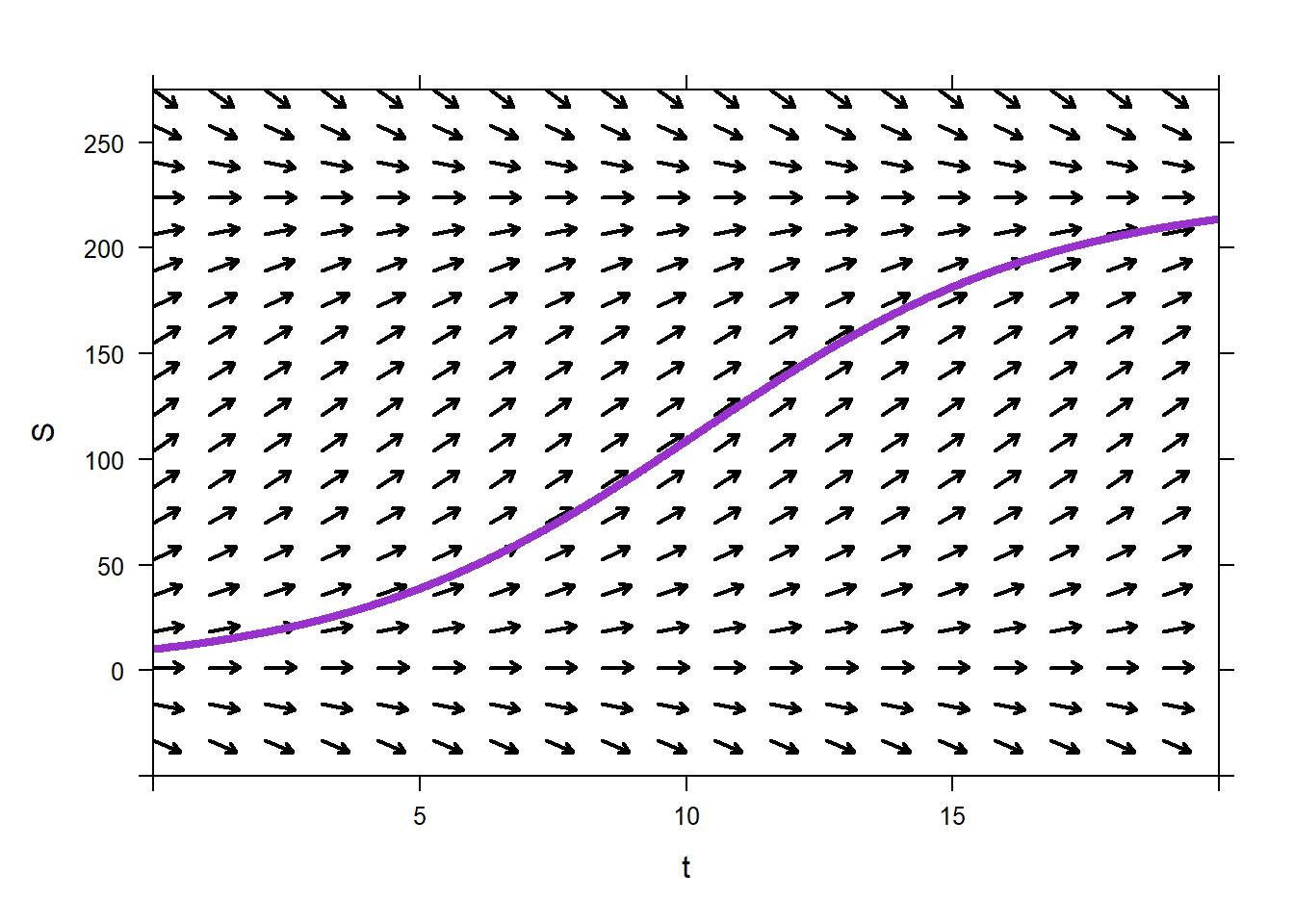 From the direction field, we can see that if the initial population is anywhere between 0 and 225 squirrels, the population follows a sigmoidal path and increases towards the carrying capacity of 225. If the initial population is above 225 squirrels, then the population is predicted to decrease towards the carrying capacity of 225 squirrels. If the initial population is either 225 or 0, then the population is predicted to stay constant. If the initial population of squirrels is less than 0 squirrels, which we perhaps interpret as zombie squirrels, then the population seems to become more and more negative, which sounds like a zombie squirrel apocalypse.
We can use Euler’s method to predict the population at any time we like. If we are interested in the population after 5 weeks, we can use Euler as follows. We use the tail command to view only the last few rows of the data frame produced by Euler. We use step size of 1 day.
##           t        S
## 31 4.285714 31.78722
## 32 4.428571 32.95707
## 33 4.571429 34.16262
## 34 4.714286 35.40444
## 35 4.857143 36.68301
## 36 5.000000 37.99883
We can see that after 5 weeks the squirrel population is predicted to be roughly 40 squirrels.
From the direction field, we can see that the squirrel population will likely reach 150 squirrels sometime prior to week 20. We can predict the population out to 20 weeks, and then scan our results to see at what time the population reaches 150.
##           t        S
## 88 12.42857 146.5342
## 89 12.57143 148.7243
## 90 12.71429 150.8851
## 91 12.85714 153.0151
## 92 13.00000 155.1132
Sometime around time \(t=12.7\) weeks the population of squirrels is expected to reach 150.
8.2.1 Logistic Equation with Harvesting
The logistic equation can be modified to include a variety of factors other than the natural reproductive rate of the population (measured with \(k\)) and the resource limitations of the environment (measured with \(M\)). One common modification is to include some type of harvesting.
The logistic equation with harvesting is \[\frac{dP}{dt}=kP\left(1-\frac{P}{M}\right)-h.\] The parameters \(k\) and \(M\) are unchanged from the logistic equation. The parameter \(h\) measures the rate, in population per time, at which individuals are removed from the population due to hunting (\(h>0\)) or added to the population (\(h<0\)).
8.2.1.1 Example
Continuing with the squirrel example above, imagine that a hawk has moved into the park where the squirrels are living. The hawk is an efficient hunter, and he eats 2 squirrels each day, or 14 squirrels per week.
A logistic equation to model this situation is \[S' = 0.3S\left( 1 - \frac{S}{225} \right) - 14.\]
Again, we can use direction fields to understand the nature of solutions to this differential equation. This code produces warnings, but the results are correct.
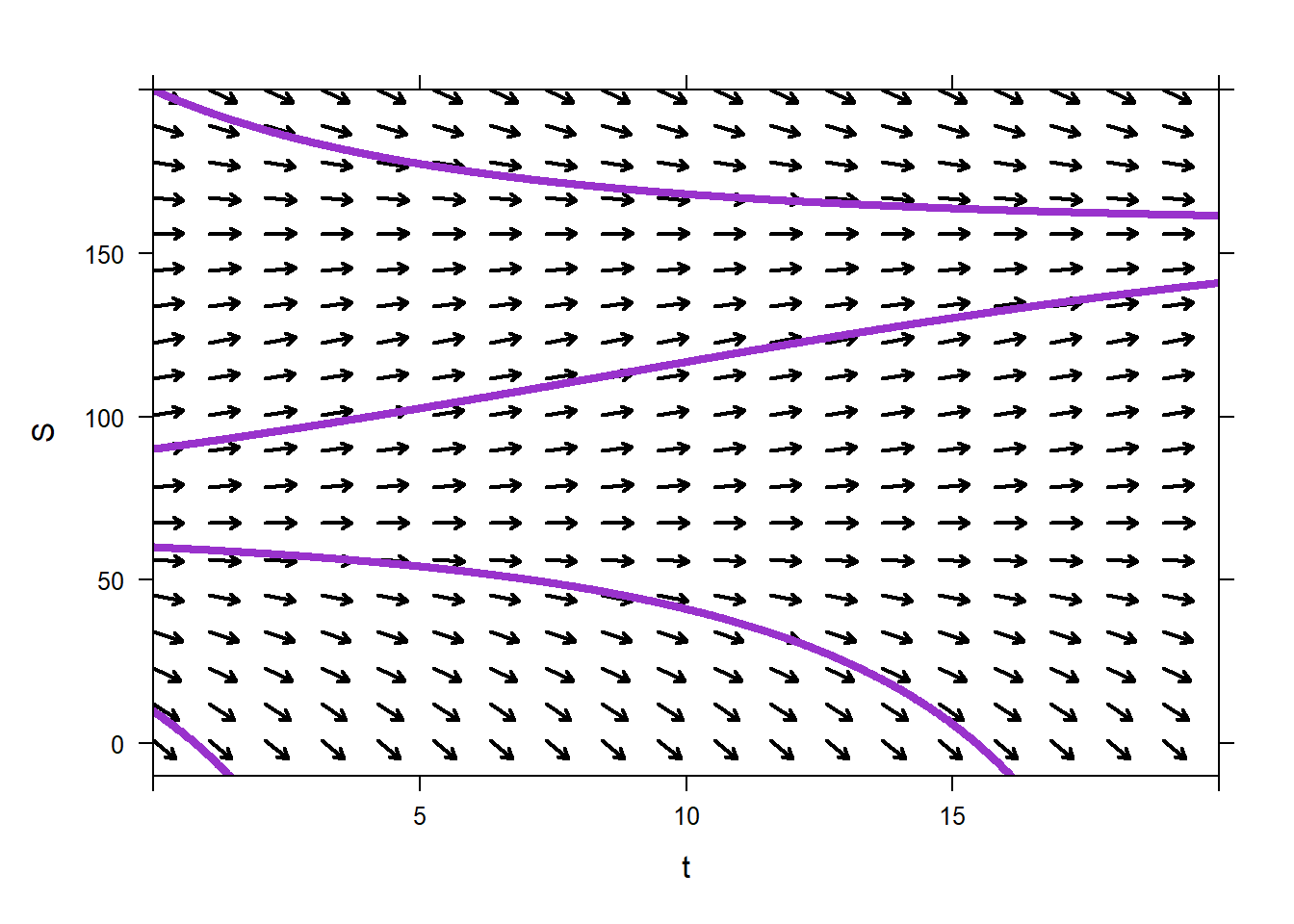
We can see that the impact of the hawk has changed the squirrel dynamics considerably. An initial population of 10 squirrels now results in over-hunting by the hawk; the squirrels go extinct. Indeed, there is a critical number of squirrels, somewhere around 65 squirrels, below which the population will not survive. However, if the initial population of squirrels is above the critical population, the squirrel population increases to happy(ish) coexistence with the hawk with around 160 squirrels. We will examine the nature of these two important populations in the next chapter.
8.3 Falling Bodies
8.3.1 No Wind Resistance
Consider an object falling towards the earth. Let the height of the object at time \(t\) be \(h(t)\), and let the velocity of the object at time \(t\) be \(v(t)\). Newton’s second law tells us that \[ma=F,\] where \(m\) is the mass of the object, \(a\) is the acceleration experienced by the object, and \(F\) is the net force acting on the object. Assume that there is no wind resistance. In that case, the only force acting on the object is gravity. The force of gravity acting on the object is \(mg\), where \(m\) is the mass of the object and \(g\) is the acceleration due to gravity.
With this in mind, we have \[ma=mg,\] and so \[a=g.\] Now, we know that the acceleration the object experiences is the derivative of velocity, so \[v'=g.\] Since \(g\) is a constant, this is a pure-time ODE that we can solve by integrating. \[v=gt+C_1.\] Further, we know that the object’s velocity is the derivative of its height, so \[h'=v=gt+C_1.\] This is once again a pure-time ODE that we can solve by integration. \[h=g\frac{t^2}{2}+C_1t+C_2.\] If we know our initial conditions, say that \(h(0)=h_0\) and \(v(0)=v_0\), we can solve for the constants above and get \[h(t)=g\frac{t^2}{2}+v_0t+h_0.\] This matches the formula familiar to many students of high school physics. The formula, however, is a consequence of the fundamental assumptions of Newton’s second law and no wind resistance. Those assumptions are naturally expressed as an ODE.
8.3.1.1 Example
A bowling ball is dropped from an airplane with height 5,000 meters. Assuming that the ball was tossed slightly upward from the plane with initial velocity 2 meters/second, and assuming that wind resistance does not impact the motion of the ball, how long will it take the bowling ball to hit the earth?
Solution Let \(t=0\) correspond to the time at which the ball was dropped, and assume that time is in seconds. Since there is no wind resistance, an IVP for the velocity of the ball is \[v'=-9.8,\quad v(0)=2.\] Here we are using \(g=-9.8\) meters/second\(^2\), the negative sign is to indicate that the acceleration happens in the downward direction.
We can solve the IVP via integration to get \[v=-9.8t+C_1.\] The initial condition \(v(0)=2\) determines \(C_1\). \[2=v(0)=-9.8\cdot 0 + C_1 = C_1.\] Therefore, \[v=-9.8t+2.\] From \(v\) we can find a formula for \(h\) by solving the IVP \[h'=v=-9.8t+2,\quad h(0)=5000.\] \[h=-9.8\frac{t^2}{2}+2t+C_2.\] Using the initial condition, \[5000=h(0)=-9.8\frac{0^2}{2}+2\cdot 0 +C_2=C_2.\] Therefore \[h=-9.8\frac{t^2}{2}+2t+5000.\] Now we can solve for the time at which the height of the bowling ball is zero using the quadratic formula. \[\begin{aligned} &0=h(t)=-9.8\frac{t^2}{2}+2t+5000\\ &t=\frac{-2\pm \sqrt{2^2-4\cdot (-9.8)\cdot 5000}}{2\cdot(-9.8)}\\ &t=-22.486\text{ or } t=22.69. \end{aligned} \] Since negative time does not make sense in this context, we take the solution \(t=22.69.\)
Instead of using algebra to solve for \(t\), we could have used the solution to our IVP along with findZeros.
##           t
## 1 -22.48589
## 2  22.68997
8.4 Newton’s Law of Cooling
Consider an object with changing temperature. Call the temperature of the object at time \(t\) \(T(t)\). Suppose that the temperature of the object is changing because it is situated in an environment with temperature \(T_A\) (for ambient temperature), and assume that the temperature of the environment does not change. One might think of the object as a nice cool glass of lemonade sitting in a warm room. The temperature of the lemonade will change due to the warm environment, will the temperature of the room will not change appreciably. Newton’s Law of Cooling (though it works just as well for heating) says that the rate of change of the temperature of the object is proportional to the temperature difference between the environment and the object. Mathematically, this means that \[T'=\lambda(T_A-T).\] \(\lambda>0\) is coefficient of proportionality that determines exactly how quickly the object cools (heats). If \(\lambda\) is large then the object cools (heats) quickly. If \(\lambda\) is small then \(T'\) is small, and we can think of the object as well insulated; it does not change temperature quickly even though there may be a substantial temperature difference with the environment.
8.4.1 Example
A mug full of coffee sits, sadly forgotten, on a counter top near the coffee machine. The coffee was initially delightfully hot, with a temperature of 120\(^\circ\)F. The temperature of the room in which the coffee sits is a comfortable 70\(^\circ\)F. Assuming that the heat transfer coefficient is \(\lambda = 0.09\) minute\(^{-1}\),
- write an IVP describing the temperature of the coffee,
- determine the temperature of .he coffee after a long time, and
- determine the time at which the coffee will become much less desirable, 90\(^\circ\) F.
Solution The IVP describing this situation is \[T'=0.09(70-T),\,T(0)=120.\] If we plot the direction field for this ODE we see that regardless of the initial condition, the coffee will approach room temperature, 70\(^\circ\)F.
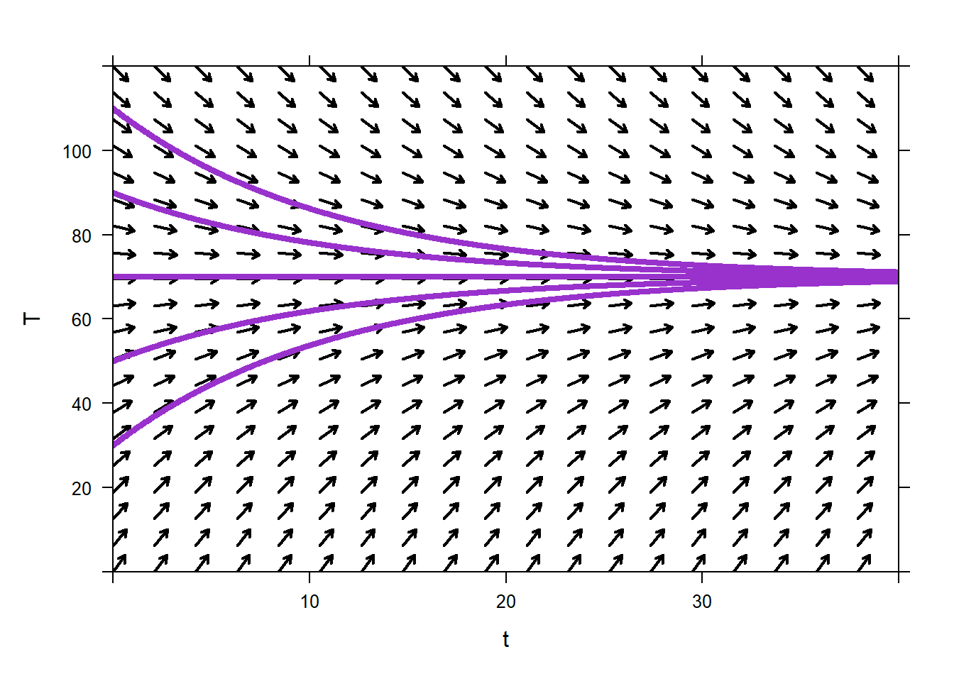
Figure 8.1: A Direction Field for the Newton’s Law of Cooling Example.
In order to find the time at which the coffee reaches 90\(^\circ\) we can solve the differential equation for \(T\) (it is separable) and then solve \(90=T\) for time. \[\begin{aligned} &\frac{dT}{dt}=0.09(70-T)\\ &\frac{1}{70-T}\frac{dT}{dt}=0.09\\ &\int \frac{1}{70-T}\frac{dT}{dt}\,dt=\int 0.09\,dt\\ &\int \frac{1}{70-T}dT=0.09t+C_1\\ &-\ln(70-T)=0.09t+C_1\\ &\ln(70-T)=-0.09t-C_1\\ &70-T=e^{-0.09t-C_1}\\ &T=70-e^{-0.09t-C_1}\\ &T=70-e^{-0.09t}e^{-C_1}\\ &T=70-Ce^{-0.09t}\\ \end{aligned}\] The initial condition is \(T(0)=120\), so \[\begin{aligned} &120=T(0)=70-Ce^{-0.09\cdot 0}=70-C\\ &C=-50. \end{aligned}\] So \[T=70+50e^{-0.09t}.\] Now we solve for the time at which the coffee reaches 90\(^\circ\)F. \[\begin{aligned} &90=70+50e^{-0.09t}\\ &20=50e^{-0.09t}\\ &\frac{20}{50}=e^{-0.09t}\\ &\ln\left(\frac{20}{50}\right)=-0.09t\\ &\frac{1}{-0.09}\ln\left(\frac{20}{50}\right)=t\approx 10.18. \end{aligned} \] The coffee reaches 90\(^\circ\)F after approximately 10.18 minutes.
Alternatively, we could use Euler to approximate the solution to the IVP, and then look for a time at which the coffee reaches around 90\(^\circ\)F.
##        t        T
## 101 10.0 90.24582
## 102 10.1 90.06361
## 103 10.2 89.88304
8.5 Further Examples
8.5.1 Bacterial Growth
During a summer picnic, potato salad is left outside on a table. The bacteria in the salad reproduce rapidly as the potato salad warms. If the bacteria population doubles every 20 minutes, how long will it take 1,000 bacteria to become \(10^{12}\) bacteria?
We start by modeling the rate of change of the bacteria population. Let \(B(t)\) represent the bacteria population and let \(t\) be the independent variable measuring time in hours. The rate of change of bacteria is proportional to the number of bacteria, so the model is
\[B^{'} = kB.\]
We can calculate the general solution to this autonomous ODE as we did in Section 8.1.1. The solution is
\[B(t) = Ce^{kt}.\]
The initial condition is given as \(B(0) = 1000\), and we can calculate the value for \(C\) as
\[\begin{aligned}
&1000 = B(0) = Ce^{k\cdot 0}\\
&C = 1000.\end{aligned}\]
We calculate the growth rate, \(k\), by applying the fact that the population doubles every 20 minutes (1/3 hours). We could use the formula given in 8.1.1 directly, \[\begin{aligned} &\text{doubling time}=\frac{\ln(2)}{k}\\ &\frac13=\frac{\ln(2)}{k}\\ &k=3\ln(2)\approx 2.08. \end{aligned} \] Alternatively, we know that \[B=1000e^{kt}.\] Since the population doubles every 1/3 hour, at time 1/3 the population will be 2000. We can use this information to solve for \(k\) directly. \[\begin{aligned} &2000=B(1/3)=1000e^{k\cdot 1/3}\\ &2=e^{k\cdot 1/3}\\ &\ln(2)=k\cdot 1/3\\ &\frac{\ln(2)}{1/3}=k\approx 2.08.\end{aligned}\]
Either way, we end up with \(k=2.08\) so that \[B=1000 e^{2.08 t}.\] Finally, we want to solve for the value of \(t\) when \(B(t) = 10^{12}\).
\[\begin{aligned} &10^{12} = 1000e^{2.08 t}\\ &10^9= e^{2.08 t}\\ &\ln(10^9) = 2.08 t\\ &t = \frac{\ln(10^9)}{2.08} \approx 9.96 \text{ hours.}\end{aligned}\] The initial population of 1000 bacteria grows to 1 trillion bacteria in just under 10 hours.
8.5.2 Learning Rates
For some subjects the rate at which a person learns new material is proportional to the proportion he or she has left to learn. What is a model for this type of learning?
Let the proportion already learned by given by \(L(t)\) where \(t\) is time in hours. Note that this proportion is bounded between 0 (knowing nothing about the subject) and 1 (knowing everything about the subject). Thus, \(0 \leq L(t) \leq 1\) for any value of \(t\). An appropriate model is
\[L^{'} = k(1 - L)\]
where \(k\) is the learning rate. This model says, “The rate of change of learning is proportional to the amount remaining to be learned.” Amounts can be scaled to proportions.
8.5.3 Disease Spread with the Logistic Equation
Consider a student with the flu returns to an isolated college campus with 4000 students. Assume all the students interact equally and on a constant basis, and all students will end up catching the flu once. What is a model/IVP for the number of people who have been infected by the flu?
In this case, the flu will spread exponentially as the college students interact and there are many students left to catch the flu. However, the disease will slow down as the students gain immunity. Each infected person will infect some proportion of those with whom he or she interacts. However, the number of students who have been infected is limited to 4000. This situation can be modeled with the logistic equation.
Let \(F(t)\) be the number of people who have caught the flu at some point where \(t\) is time measured in days. The logistic equation gives the model
\[F^{'} = kF\left( 1 - \frac{F}{4000} \right)\]
where \(k\) represents the rate at which the flu spreads. This model says, “The rate of change of students who have contracted the flu is proportional to the product of the number of students who have already caught the flu and the number who have not yet caught the flu.” The product represents the interaction between those with the flu and those without the flu.
8.5.4 Radioactive Decay
Initially 1g of a radioactive substance is present. After 12 hours, the mass decreased by 2%. If the rate of decay is proportional to the amount of the substance present at time \(t\), then how much of the radioactive substance is remaining after 1 week?
Let \(S(t)\) be the amount of substance in milligrams where \(t\) is time measured in days. Since the rate of change is proportional to the amount of substance and the substance is decaying, we can use
\[S^{'} = k S,\quad S(0)=1000.\]
where \(k\) is the rate of decay measured in \(days^{- 1}\). As we saw in 8.1.2, the solution to this problem is \[S=1000e^{k t}.\]
After 1/2 day the substance has been reduced by 2%. Therefore, we can find the decay rate as
\[\begin{aligned}
&0.98 \cdot 1000 = S(1/2) = 1000e^{k\cdot 0.5 }\\
&0.98 = e^{0.5k}\\
&\ln(0.98) = 0.5k\\
&k = \frac{1}{0.5}\ln(0.98)\approx -0.0404.
\end{aligned}\]
If we had desired, we could have used findZeros to solve \(0.98\cdot 1000 -1000 \cdot e^{k\cdot 0.5} =0\) for \(k\). We are using the option roundDigits to provide more than two decimal places of accuracy.
##         k
## 1 -0.0404
Either way \(k\) is determined, the complete model for the decaying substance is
\[S(t) = 1000e^{-0.0404 t}.\]
Now we evaluate the function at \(t = 7\) days.
\[S(7) = 1000e^{-0.0404 \cdot 7}\approx 753.67 \text{mg}.\]
Of the original 1000mg, there are 753.67mg remaining after 1 week.
8.6 Exercises
- A cadet can invest part of his/her Firstie car loan. Assume the money can be placed in a secure investment that earns 6% compounded continuously. Note: interest rates are always given as annual rates.
- Develop a differential equation that models the value of the investment, \(P\),
- Given the initial value, \(P_{0} = \$ 12,000\), find the investment’s value as a function of time,
- State the investment’s value after a 25-year AF career, i.e. after 26 years.
- Consider that a modern SUV’s value, \(V\), changes at a rate that is directly proportional to its current value. The constant of proportionality for the SUV’s decreasing value is \(\lambda = 0.023\) months\(^{- 1}\).
- Provide the differential equation model for the SUV’s value, \(V\),
- Given the initial value, \(V_{0} = \$ 56,000\), provide the SUV’s value as a function of time, and
- Provide the approximate value of the SUV after 60 months.
- A Ferrari 428 has a top speed of 195 mph, and its acceleration is proportional to the difference between its current speed and 195 mph.
- Provide a differential equation model for the speed, \(v\), of the Ferrari,
- Given the Ferrari starts at rest and can reach 100 mph in 7 seconds, find the function that represents the Ferrari’s speed, \(v(t)\),
- Determine the amount of time required for the Ferrari to reach 180 mph.
- The population of deer on the Air Force Academy does not face any natural predators. The population of deer, \(D\), changes at a rate proportional to the population. The growth rate of deer is \(k = 0.4\) year\(^{- 1}\), and we assume there is no limit to the number of deer USAFA can hold. Each year, hunters harvest 35 deer.
- Provide a differential equation model for the number of deer, \(D\),
- Given an initial deer population of 100, state the deer population as a function of time,
- State the deer population after 5 years.
- Metabolism of acetaminophen (Tylenol) is an important consideration for patients. The rate at which acetaminophen is metabolized is directly proportional to the amount of acetaminophen, \(A\), in a person’s body. The half-life of this drug is 2.5 hours. Complete these 3 steps:
- Provide the differential equation model for the amount of acetaminophen, \(A\), in a person’s body,
- Given the initial amount, \(A_{0} = 500mg,\ \)provide the amount of acetaminophen as a function of time,
- Provide the length of time required for the amount to fall below 70mg.
- Consider the population of Cutthroat Trout in the Colorado River between Grand Junction and Fruita (~10 miles). The population of Cutthroat Trout, \(T\), changes at a rate proportional to the population when the population is not near the river’s carrying capacity. The growth rate of cutthroat is \(k = 2\) year\(^{- 1}\), and the 10 miles of river can hold a maximum of 12000 fish.
- Provide the differential equation model for the Cutthroat population, \(T\), along this 10-mile stretch of river,
- Plot the direction field for the model and estimate the long-term population of trout in the riverm
- Given an initial population of 500 Cutthroat, use the
Euleror algebra to estimate how long it will take for the population of fish to reach 11000.
- Continue using the background information from the previous problem. Complete these 3 steps:
- Modify your model from to include the fact that fishermen and Osprey catch and remove approximately 4000 Cutthroat each year,
- Plot a direction field for this model. Estimate the minimum sustainable population of Cutthroat in this river?
- (more difficult) What is the maximum number of Cutthroat that can be taken by fishermen and Osprey each year?