Chapter 10 Systems of 1st Order ODEs
10.1 Introduction to Systems of ODEs
Thus far, we have considered 1st order ordinary differential equations as individual items. Just as in algebra we can think about solving systems of simultaneous equations, and doing so broadens the scope of problem we can solve, we can consider solving systems of differential equations. All of the unknown functions are still functions of a single independent variable. We will continue to use \(t\) as the independent variable. Our investigation into systems of 1st order ODE’s will generally have 2 (sometime 3) dependent functions. For example:
\[\begin{aligned} x'(t) &= f(x,y,t) \\ y'(t) &= g(x,y,t). \end{aligned}\]
where \(x\) and \(y\) are the unknown functions of \(t\), and the right-hand sides, \(f\) and \(g\), give the rates of change for \(x\) and \(y\), respectively.
Given this basic form for a system of 1st order ODE’s, we see that the solution is now a set of two functions, both \(x(t)\) and \(y(t)\). Let’s consider a simple example: \[\begin{aligned} x' &= y \\ y' &= x \end{aligned}\] with \(t\) as the independent variable. We seek the pair of functions, \(x(t)\) and \(y(t)\), that satisfy the system above. Certainly this problem is not as easy as \(y' = y\), but it is closely related. We can immediately see one solution: \[\begin{aligned} x(t) &= C_{1}e^{t} \\ y(t) &= C_{1}e^{t} \end{aligned}\]
where \(C_{1}\) is any constant. Notice the solution must contain both functions. We can verify this solution just as we did with a single 1st order ODE: \[\begin{aligned} x' &= \frac{d}{dt}\left[x(t)\right]=\frac{d}{dt}\left[C_1e^t\right]=C_{1}e^{t} = y(t). \\ y' &= \frac{d}{dt}\left[y(t)\right]=\frac{d}{dt}\left[C_1e^t\right]=C_{1}e^{t} = x(t). \end{aligned}\]
Also, as we recall from our introduction to ODE’s, this solution represents an entire family of solutions. Any real valued constant, \(C_{1}\), gives a correct solution.
There is another solution for our system. In this text we will not derive solutions to 1st order ODE’s. However, it is important to realize that, in general, there are an many solutions for these systems as there are differential equations. In this example we have 2 ODE’s, and we can expect to find 2 solutions. Here is the second solution: \[\begin{aligned} x(t) &= C_{2}e^{- t} \\ y(t) &= - C_{2}e^{- t} \end{aligned}\]
where \(C_{2}\) is any constant. Again, the solution must contain both functions, and we can verify the solution by applying the functions to the ODEs:
\[\begin{aligned} x' &= - C_{2}e^{- t} = y(t) \\ y' &= C_{2}e^{- t} = x(t) \end{aligned}\]
Because we have two solutions, we often number these solutions. A common form for the solutions to a system of 1st order ODEs looks like this:
| Solution #1 | Solution #2 |
|---|---|
| \[\begin{aligned} x_{1}(t) &= C_{1}e^{t} \\ y_{1}(t) &= C_{1}e^{t} \end{aligned}\] | \[\begin{aligned} x_{2}(t) &= C_{2}e^{- t} \\ y_{2}(t) &= - C_{2}e^{- t} \end{aligned}\] |
These two solutions, each being a set of two functions \(x(t)\) and \(y(t)\), can be combined into a single, general solution. We create the general solution by taking a linear combination of the individual solutions. The specific procedure for creating the general solution is not important here. We simply state the general solutions as: \(\begin{aligned} x(t) &= C_{1}e^{t} + C_{2}e^{- t}, \\ y(t) &= C_{1}e^{t} - C_{2}e^{- t}. \end{aligned}\)
Again, we can verify that the general solution solves the differential equations. \[\begin{aligned} x' &= C_{1}e^{t} - C_{2}e^{- t} = y(t) \\ y' &= C_{1}e^{t} + C_{2}e^{- t} = x(t) \end{aligned}\] Note that the linear combination of the individual solutions gives a complete solution to the problem. This general solution is still a family of solutions, but it has 2 constants instead of just 1 as we saw earlier.
In order to solve for the constants, \(C_{1}\) and \(C_{2}\), we apply initial conditions (IC’s) as we did with a single ODE. The IC’s must be applied simultaneously. Consider these initial conditions applied to our example: \(x(0) = 3\) and \(y(0) = 1\). Applying these conditions to the general solution yields: \[\begin{aligned} 3&=x(0) = C_{1}e^{0} + C_{2}e^{- 0} \\ 1&=y(0) = C_{1}e^{0} + C_{2}e^{- 0} \end{aligned}\]
Simplifying
\[\begin{aligned}
3 &= C_{1} + C_{2} \\
1 &= C_{1} - C_{2}
\end{aligned}\]
This system of algebraic equations can be solved by hand or using findZeros for systems of equations.
##   C1 C2
## 1  2  1
The values for the constants has identified a single solution out of the family represented by the general solution. The particular solution to the initial value problem (IVP) is:
\[\begin{aligned} x(t) &= 2e^{t} + e^{- t} \\ y(t) &= 2e^{t} - e^{- t} \end{aligned}\]
The particular solution satisfies both the system of ODE’s and the set of initial conditions.
Finding solutions to systems of 1st order ODEs is possible on occasion, but most systems of ODEs cannot be solved analytically. To learn more about analytical solutions to ODEs, we recommend the reader take a course in Ordinary Differential Equations.
10.1.1 Example #1
Consider the system of ODE \[\begin{aligned} x' &= - 3y \\ y' &= 2x - 5y. \end{aligned}\] Does \[\begin{aligned}x &= 3e^{- 2t} \\ y &= 2e^{- 2t} \end{aligned}\] solve this system of ODE?
Solution
For System A pair #1, we have: \(x' = - 6e^{- 2t}\) and \(y' = - 4e^{- 2t}\). Checking both sides of the system yields:
LHS:
\[\begin{aligned} x' &= - 6e^{- 2t} \\ y' &= - 4e^{- 2t} \end{aligned}\]
RHS: \[\begin{aligned} &- 3y = - 3 \cdot 2e^{- 2t} = - 6e^{- 2t} \\ &2x - 5y = 2 \cdot 3e^{- 2t} - 5 \cdot 2e^{- 2t} = - 4e^{- 2t} \end{aligned}\]
We can see that LHS=RHS, so the pair of functions \(x = 3e^{- 2t}\), \(y = 2e^{- 2t}\) is a solution to the system of ODEs.
10.1.2 Example #2
Consider the system of ODE \[\begin{aligned} x' &= - 3y \\ y' &= 2x - 5y. \end{aligned}\] Does \[\begin{aligned} x &= e^{- 3t} \\ y &= 2e^{- 3t} \end{aligned}\] solve this system?
Solution
Checking both sides of the system yields:
LHS:
\[\begin{aligned} x' &= - 3e^{- 3t} \\ y' &= - 6e^{- 3t} \end{aligned}\]
RHS:
\[\begin{aligned} &- 3y = - 3 \cdot 2e^{- 3t} = - 6e^{- 3t} \\ &2x - 5y = 2 \cdot e^{- 3t} - 5 \cdot 2e^{- 3t} = - 8e^{- 3t}. \end{aligned}\]
Since LHS is not equal to RHS, the function pair \(x = e^{- 3t}\), \(y = 2e^{- 3t}\) does not solve the system of ODEs.
10.1.3 Example #3
Consider the system of ODE \[\begin{aligned} u' &= u - 5v \\ v' &= u - v. \end{aligned}\] Does \[\begin{aligned} u &= 5\sin(2t) \\ v &= \sin(2t) - 2\cos(2t) \end{aligned}\] solve this system?
Solution
Checking both sides of the system yields:
LHS: \[\begin{aligned} u' &= 10\cos(2t) \\ v' &= 2\cos(2t) + 4\sin(2t) \end{aligned}\]
RHS: \[\begin{aligned} u - 5v &= 5\sin(2t) - 5(\sin(2t) - 2\cos(2t)) = 10\cos(2t) \\ u - v &= 5\sin(2t) - (\sin(2t) - 2\cos(2t)) = 4\sin(2t) + 2\cos(2t) \end{aligned}\]
Since LHS=RHS, the function pair \(u = 5\sin(2t)\), \(v = \sin(2t) - 2\cos(2t)\) solves the system of ODE.
10.1.4 Example #4
\[\begin{aligned} u' &= u - 5v \\ v' &= u - v. \end{aligned}\] Does \[\begin{aligned} u &= 2\sin(2t) + 4\cos(2t) \\ v &= 2\sin(2t) \end{aligned}\] solve this system of ODE?
Solution
Checking both sides of the system yields:
LHS: \[\begin{aligned} u' &= 4\cos(2t) - 8\sin(2t) \\ v' &= 4\cos(2t) \end{aligned}\]
RHS:
\[\begin{aligned} u - 5v &= 2\sin(2t) + 4\cos(2t) - 5 \cdot 2\sin(2t) = - 8\sin(2t) + 4\cos(2t) \\ u - v &= 2\sin(2t) + 4\cos(2t) - 2\sin(2t) = 4\cos(2t) \end{aligned}\]
Since LHS=RHS, the function pair \(u = 2\sin(2t) + 4\cos(2t)\), \(v = 2\sin(2t)\) solves the system of ODE.
10.1.5 Example #5
Consider the system of ODEs \[\begin{aligned} u' &= u - 5v\\ v' &= u - v. \end{aligned}\]
This system has the general solution
\[\begin{aligned} u &= \left(C_{1} - 5C_{2}\right)\sin(2t) + 2C_{1}\cos(2t) \\ v &= \left(C_{1} - C_{2}\right)\sin(2t) + 2C_{2}\cos(2t). \end{aligned}\]
Solve for the constants \(C_{1}\) and \(C_{2}\) given the initial conditions: \(u(0) = 2\) and \(v(0) = - 4\).
We proceed by substituting the ICs into the general solution: \[\begin{aligned} &2=u(0) = \left( C_{1} - 5C_{2} \right)\sin(2 \cdot 0) + 2C_{1}\cos(2 \cdot 0) \\ &2 = 2C_{1}\\ &C_{1} = 1. \\\end{aligned}\]
\[\begin{aligned} &-4=v(0) = \left( C_{1} - C_{2} \right)\sin(2 \cdot 0) + 2C_{2}\cos(2 \cdot 0) \\ &- 4 = 2C_{2}\\ &C_{2} = - 2. \end{aligned}\]
Using the constants, we build the particular solution.
\[\begin{aligned} u &= \left( 1 - 5 \cdot (-2) \right)\sin(2t) + 2 \cdot 1 \cdot \cos(2t) \\ &= 11\sin(2t) + 2\cos(2t) \\ v &= \left( 1 - (-2) \right)\sin(2t) + 2 \cdot (-2) \cdot \cos(2t) \\ &= 3\sin(2t) - 4\cos(2t). \end{aligned}\]
The specific solution is: \(u(t) = 11\sin(2t) + 2\cos(2t)\) ; \(v(t) = 3\sin(2t) - 4\cos(2t)\)
Note that we could also find the constants in the specific solution using findZeros, by manually inserting \(t=0\). For example,
##   C1 C2
## 1  1 -2
10.2 Equilibrium Solutions
We focus on autonomous, systems of 1st order differential equations:
\[\begin{aligned} x'(t) &= f(x,y) \\ y'(t) &= g(x,y) \end{aligned}\]
The definition for autonomous is the same as we saw earlier. Autonomous systems of ODE’s have rates of change that do not explicitly depend on the independent variable. Thus, the rate functions, \(f(x,y)\) and \(g(x,y)\), are never functions of \(t\).
An equilibrium solution to a system of ODEs is a pair of functions, \(x\) and \(y\), that are constant and that satisfy the ODE.
10.2.1 Example #6
Consider a park in which a population of squirrels, \(S(t)\), and a population of hawks, \(H(t)\), coexist. We assume that the the squirrels are preyed upon by hawks at a rate (squirrels/time) jointly proportional to both the number of squirrels and the number of hawks. We assume that the hawks reproduce at rate jointly proportional to the number of squirrels and hawks. In this case, a differential equation for the two populations is
\[\begin{aligned} S'&=0.3S\left(1-\frac{S}{90}\right) - 0.09SH\\ H'&=-0.5H+0.009SH. \end{aligned}\] Find all the equilibrium solutions for this system of ODE.
Solution
We seek constant values for \(S\) and \(H\) that satisfy the differential equation. If both \(S\) and \(H\) are constant, then \(S'=0\) and \(H'=0\). Therefore we need to find values of \(S\) and \(H\) that solve
\[\begin{aligned}
0&=0.3S\left(1-\frac{S}{90}\right) - 0.09SH\\
0&=-0.5H+0.009SH.
\end{aligned}\]
We could do this by hand using algebra, but it is far easier to use findZeros.
##        S     H
## 1  0.000 0.000
## 2 55.556 1.276
## 3 90.000 0.000
There are three equilibrium solutions. One equilibrium solution is \(S=0\), \(H=0\). We can interpret this to mean that our model predicts that if the population starts with \(S=0\) and \(H=0\), then the populations will never change. This makes sense.
The second equilibrium solution is more interesting. Our model predicts that if the populations of squirrels and hawks is exactly \(S=55.556\) and \(H=1.276\) then the two populations will never change. They will balance each other perfectly. Of course, it isn’t possible to have this population of squirrels and hawks, since neither species offers fractional individuals. In the next section we will explore what happens if the two populations start close to, but not exactly at, this equilibrium solution.
The final equilibrium solution is also interesting. It says that in the absence of hawks, \(H=0\), the population of squirrels will stay constant if it ever reaches exactly \(S=90\). We can interpret this as meaning that the environment itself has a natural carrying capacity for squirrels, and that in the absence of hawks the population of squirrels will satisfy a logistic equation.
10.2.2 Example #7
Consider a population of two species of tree, perhaps pine and aspen, growing in a forest. Pine and aspen trees compete for many of the same resources, sunlight, nutrients, and carbon dioxide.
Let \(P(t)\) be the population of pine tree in the forest, in thousands, and \(A(t)\) the population of Aspen, in thousands. One model for the two populations is \[\begin{aligned} A'&=0.004A(50-A-0.75P)\\ P'&=0.001P(100-P-3A) \end{aligned}\] We can find the equilibrium solutions by solving \[\begin{aligned} 0&=0.004A(50-A-0.75P)\\ 0&=0.001P(90-P-3A) \end{aligned}\] for \(A\) and \(P\).
##    A  P
## 1  0  0
## 2  0 90
## 3 14 48
## 4 50  0
We can see that there are four equilibrium solutions. One, \(A=0\), \(P=0\), means that if there are no trees in the forest, neither population will change. This makes sense.
A second equilibrium solution, \(A=0\), \(P=90\), means that if the ever has a population of 0 Aspens and 90,000 Pines, then the pine trees will out compete the aspen to such an extent that the aspen never recover. Further, the pine trees will never increase their population either.
A third equilibrium solution, \(A=50\), \(P=0\), is the reverse situation. In this situation, the aspen trees have used all the resources in the environment, and there is no more room for either pine or more aspen trees.
The fourth equilibrium solution is interesting. In this case, \(A=14\), \(P=48\), the two species have both established populations and have used all of the available resources in the environment.
10.2.3 Example #8
Consider the motion of a frictionless pendulum with length 2 meters. Let \(x(t)\) be the angle the pendulum makes with a vertical line through the pivot point, in radians, and let \(y(t)\) be the angular velocity of the pendulum, in radians per second. See the figures below.
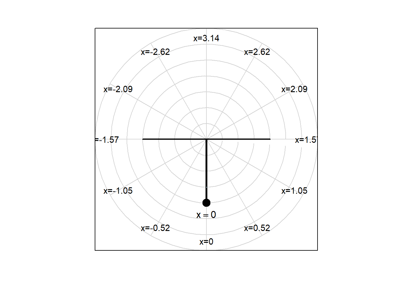
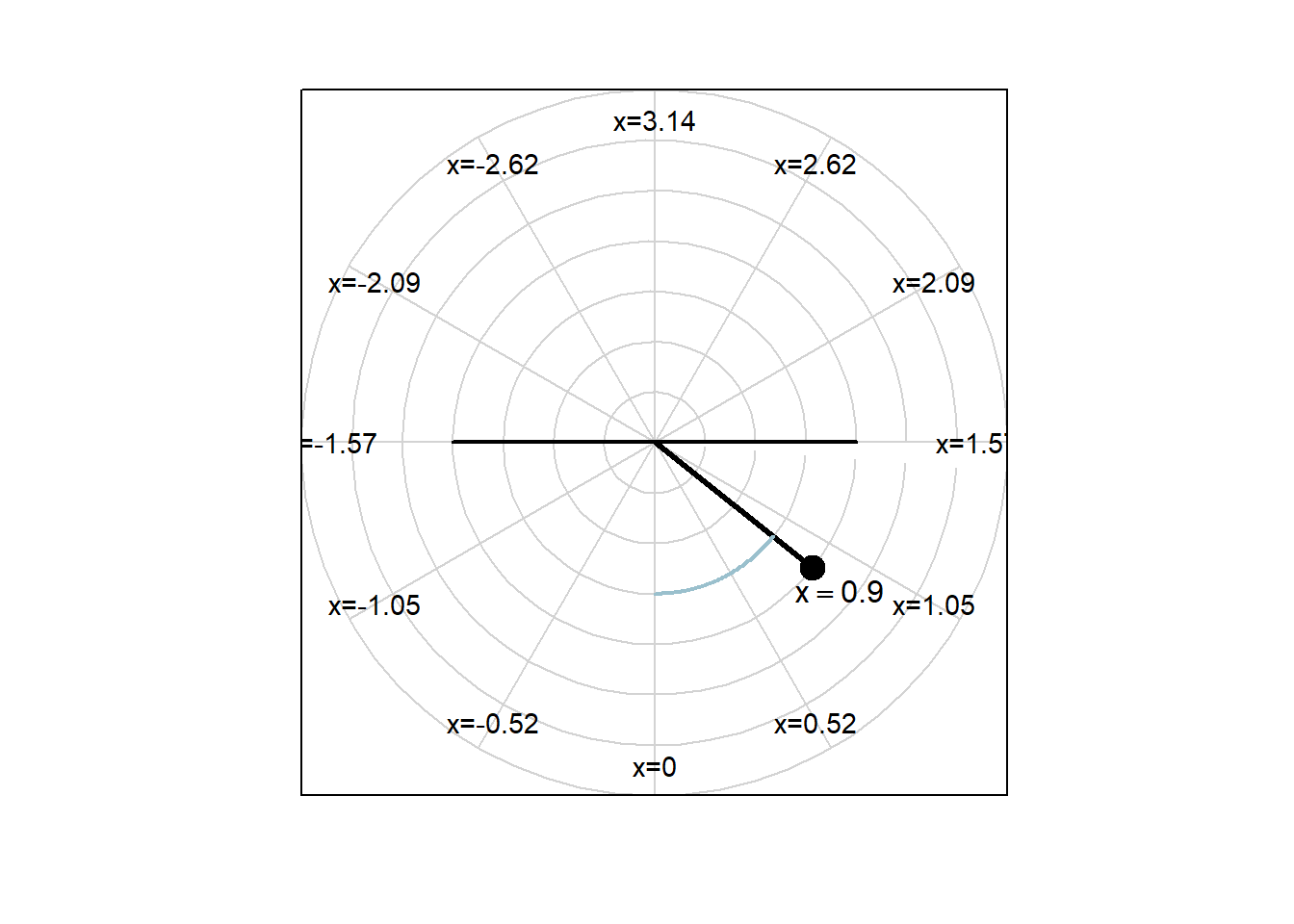
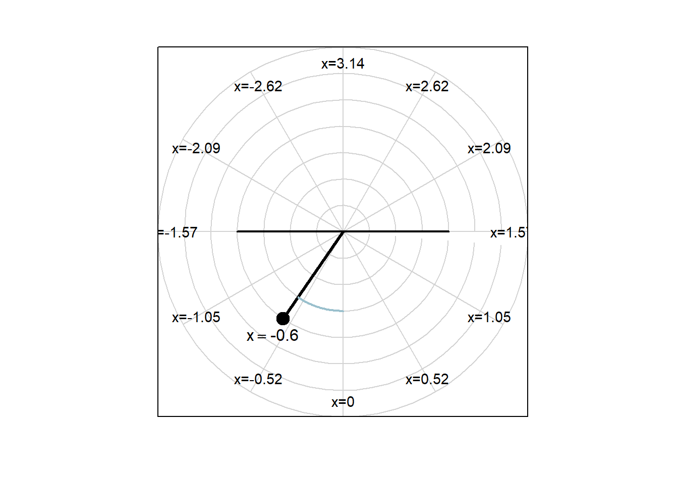 In the figures above, we can’t see \(y\), because \(y\) is the angular velocity with which the pendulum is moving.
A model that describes this motion is \[\begin{aligned} x'&=y\\ y'&=-4.9\sin(x). \end{aligned}\] The equilibrium solutions to this system of ODEs can be found by solving \[\begin{aligned} 0&=y\\ 0&=-4.9\sin(x). \end{aligned}\]
There are many equilibrium solutions to this system of equations. What position/velocity pairs do they correspond to? Do those position velocity pairs make sense?
10.2.4 Example #9
Find the equilibrium solutions for this system of 1st order ODEs \[\begin{aligned} x' &= 3y^{2} + 6y - xy \\ y' &= 3x - xy \end{aligned}\] To find the equilibrium solutions, we set the rates of change equal to zero and solve for \(x\) and \(y\). \[\begin{aligned} 0 &= 3y^{2} + 6y - xy\\ 0 &= 3x - xy \\ \end{aligned}\] Factoring, \[\begin{aligned} 0 &= y(3y + 6 - x)\\ 0 &= x(3 - y) \end{aligned}\] We see from the second equation, \(0 = x(3 - y)\), that equilibria can only occur when \(x = 0\) or \(y = 3\). We will check the first equation for each situation. With \(x = 0\), the first equation becomes \[\begin{aligned} 0 &= y(3y + 6 - 0) \\ \end{aligned}\] This has solutions \(y=0\), \(y=-2\). This gives two equilibrium solutions: \(x = 0\ ;y(t) = 0\) and \(x = 0\ ;y = - 2\).
Now we check for equilibrium solutions featuring \(y = 3\). \[\begin{aligned} 0 &= 3(3 \cdot 3 + 6 - x) \\ x &= 15 \end{aligned}\] This provides an additional equilibrium solution: \(x = 15\ ;y = 3\).
The three equilibrium solutions are: \(x = 0\ ;y = 0\) and \(x = 0\ ;y = - 2\) and \(x = 15\ ;y = 3\).
We could also find the equilibrium solutions using findZeros.
##    x  y
## 1  0 -2
## 2  0  0
## 3 15  3
10.3 The Phase Plane
In this section we will revisit many of the concepts from Section 5.1 in order to analyze the behavior of solutions to autonomous systems of equations that are not equilibrium solutions.
Consider the model for a population of squirrels and hawks from 10.2.1 \[\begin{aligned} H'&=-0.5H+0.009SH\\ S'&=0.3S\left(1-\frac{S}{90}\right) - 0.09SH. \end{aligned}\]
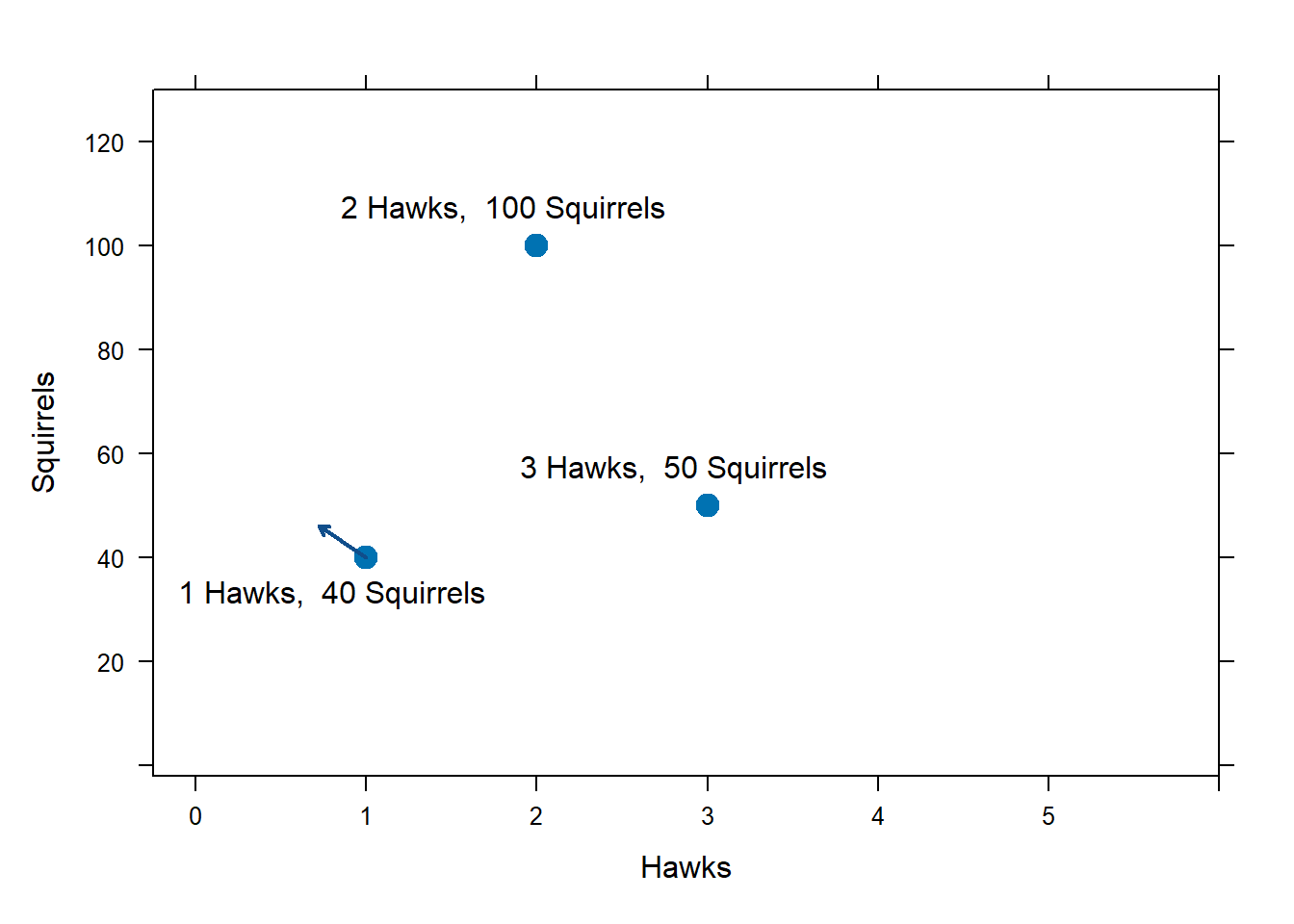
Let us draw a plane; we interpret each point in the plane as hawk population/squirrel population pair. For example, the point (1, 40) on this figure represents a hawk population of 1 and a squirrel population of 40. The point (3, 50) on this figure represents a hawk population of 3 and a squirrel population of 50. The point (2, 100) on this figure represents a hawk population of 2 and a squirrel population of 100.

Now, consider how the system of ODEs says the populations will change if the population levels reach the numbers given above.
If the current population is \(H=1\), \(S=40\), the ODE says that \(H'\) is
\[H'=-0.5H+0.009SH = -0.5\cdot 1 + 0.009\cdot 40 \cdot 1 = -0.14.\] Therefore, if the population ever reaches 1 hawks and 40 squirrels, the hawk population will be decreasing at rate -0.14 hawks per week.
We can also determine \(S'\) if the population ever becomes 1 hawks and 40 squirrels.
\[\begin{aligned}
S'&=0.3S\left(1-\frac{S}{90}\right) - 0.09SH \\
&=0.3\cdot 40 \left(1-\frac{40}{90}\right) - 0.09\cdot 40 \cdot 40 = 3.07.
\end{aligned}\]
If the population ever becomes 1 hawks and 40 squirrels, the system of ODE tells us that the squirrel population will be increasing at rate 3.07 squirrels per week.
To summarize, if the two populations ever reach this state, the hawk population will continue to decline in the near future (because in this state \(H'<0\)), and the squirrel population will increase in the near future (because in this state \(S'>0\)). To reflect this fact, we draw a vector from the current state (1,40) towards the future state, which would be down in the hawk coordinate, and up in the squirrel coordinate. In particular, we draw a vector in the direction of \((-0.14, 3.07)\), but as usual with these figures we draw the vector to a length that looks good.
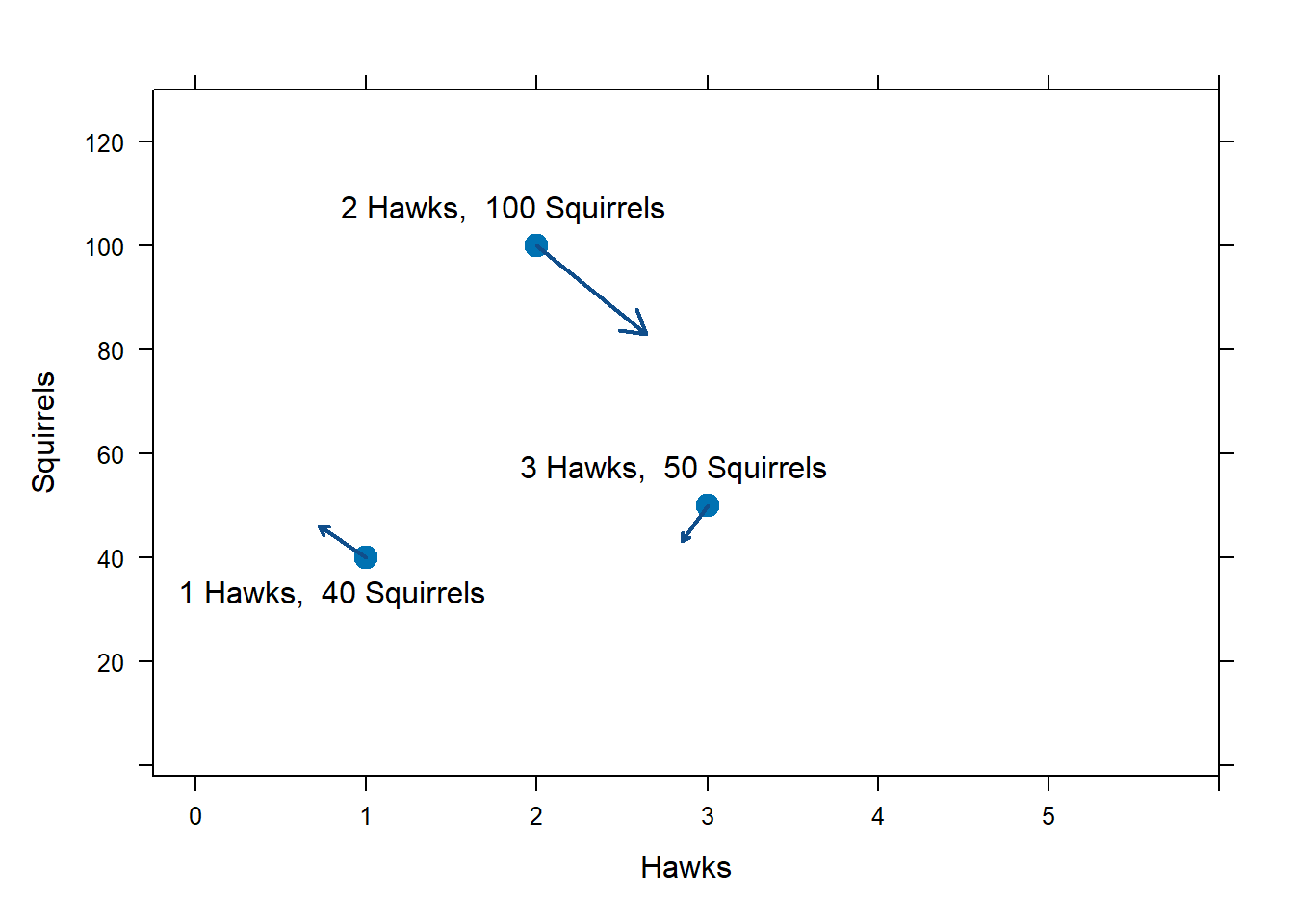
What if the population somehow reaches 3 hawks and 50 squirrels? According to the ODE, if the population reaches 3 hawks and 50 squirrels, then \[H'=-0.5H+0.009SH=0.5\cdot 3 + 0.009\cdot 50 \cdot 3 = -0.15.\] If the populations ever reach these levels, the hawk population will be decreasing at rate -0.15 hawks per week.
We can also calculate \(S'\) from this state. \[\begin{aligned} S'&=0.3S\left(1-\frac{S}{90}\right) - 0.09SH \\ &=0.3\cdot 50 \left(1-\frac{50}{90}\right) - 0.09\cdot 50 \cdot 50 = -6.83. \end{aligned}\] If the populations ever reach these levels, the squirrel population will be decreasing at rate -6.83 squirrels per week.
We record these calculations by drawing a vector in the direction of (-0.15,-6.83) originating at the current population, (3, 50). This vector tells us the direction the population will head in the future.

What if the population somehow reaches 2 hawks and 100 squirrels? According to the ODE, if the population reaches 2 hawks and 100 squirrels, then \[H'=-0.5H+0.009SH=0.5\cdot 2 + 0.009\cdot 100 \cdot 2 = 0.8.\] If the populations ever reach these levels, the hawk population will be increasing at rate 0.8 hawks per week.
We can also calculate \(S'\) from this state. \[\begin{aligned} S'&=0.3S\left(1-\frac{S}{90}\right) - 0.09SH \\ &=0.3\cdot 100 \left(1-\frac{100}{90}\right) - 0.09\cdot 100 \cdot 100 = -21.33. \end{aligned}\] If the populations ever reach these levels, the squirrel population will be decreasing at rate -21.33 squirrels per week.
We record these calculations by drawing a vector in the direction of (0.8,-21.33) originating at the current population, (2, 100). This vector tells us the direction the population will head in the future.
 If we continue in this way, we will eventually create a phase plane. A phase plane contains vectors pointing in the direction in which a solution will move.
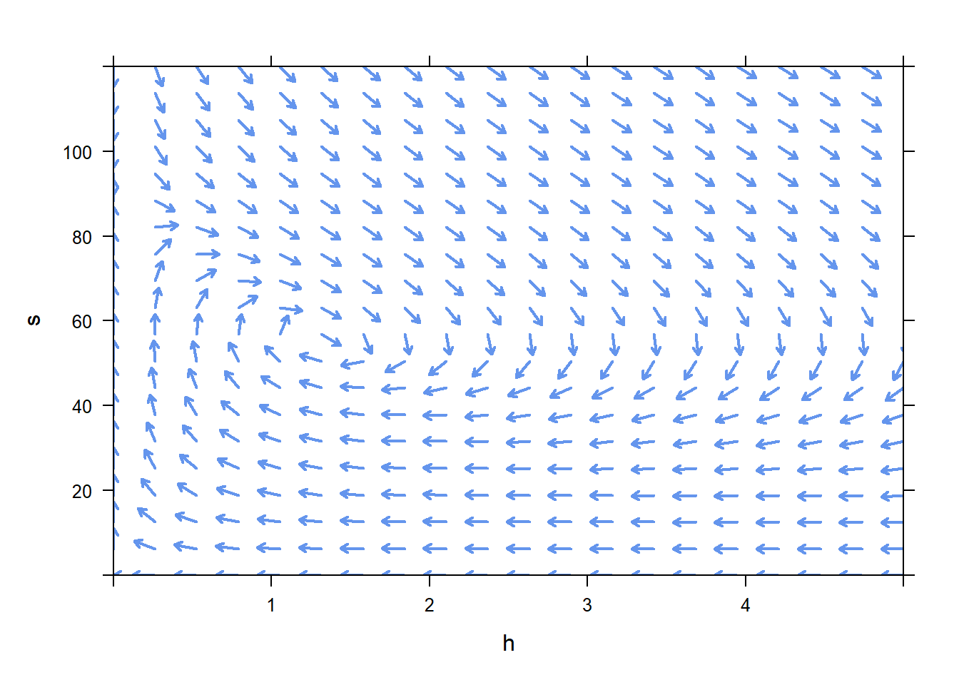
We can use plotPhasePlane to plot a phase plane for an ODE. Much like Euler or findZeros, we give all of the RHS of the ODE, collected in a vector. To plot a phase plane for
\[\begin{aligned}
H'&=-0.5H+0.009SH\\
S'&=0.3S\left(1-\frac{S}{90}\right) - 0.09SH.
\end{aligned}\]
on a portion of the phase plane with \(0<H<6\) and \(0<S<130\), we would use the following command.
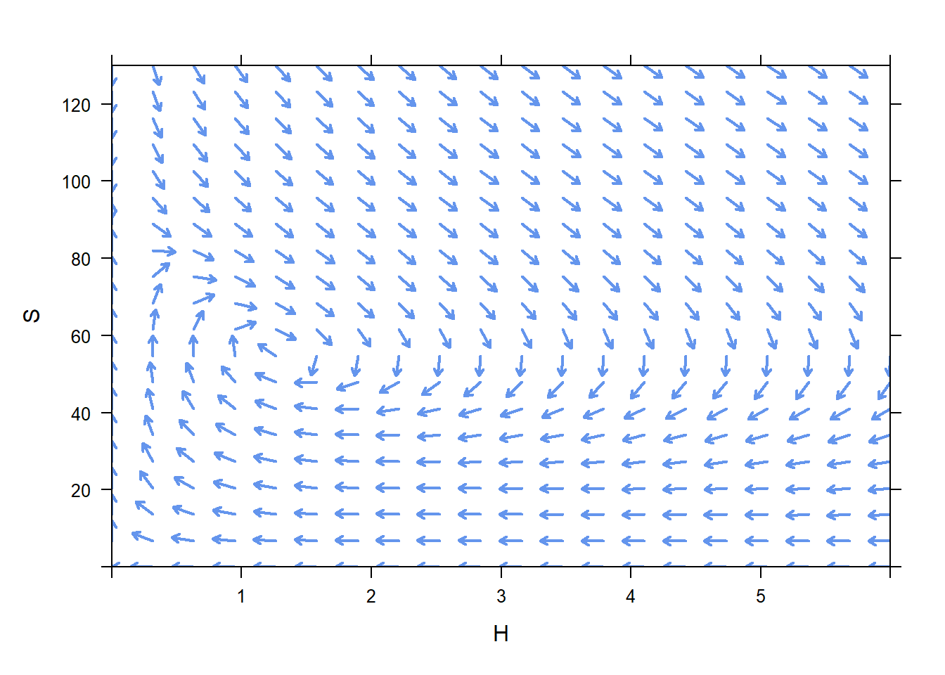
We can use the phase plane to visualize how we expect the number of hawks and squirrels to change if we start with a known population by following the arrows in the phase plane. For instance, if the initial population is 3 hawks and 100 squirrels, we expect the number of hawks to increase, and the number of squirrels to decrease. However, once the population of hawks reaches around 5.5, and the population of squirrels reaches about 85, the population of hawks looks like it will start decreasing. Once the population of hawks reaches about 3.5, and the population of squirrels reaches about 65, the population of squirrels will start increasing.
We can use plotPhasePlane to plot a trajectory that corresponds with a given initial condition. Use the option ic= to specify the initial number of hawks and squirrels.
plotPhasePlane(c(-0.5*H+0.009*S*H,
0.3*S*(1-S/90) - 0.09*S*H)~H&S,
xlim=c(0,6),ylim=c(0,130),
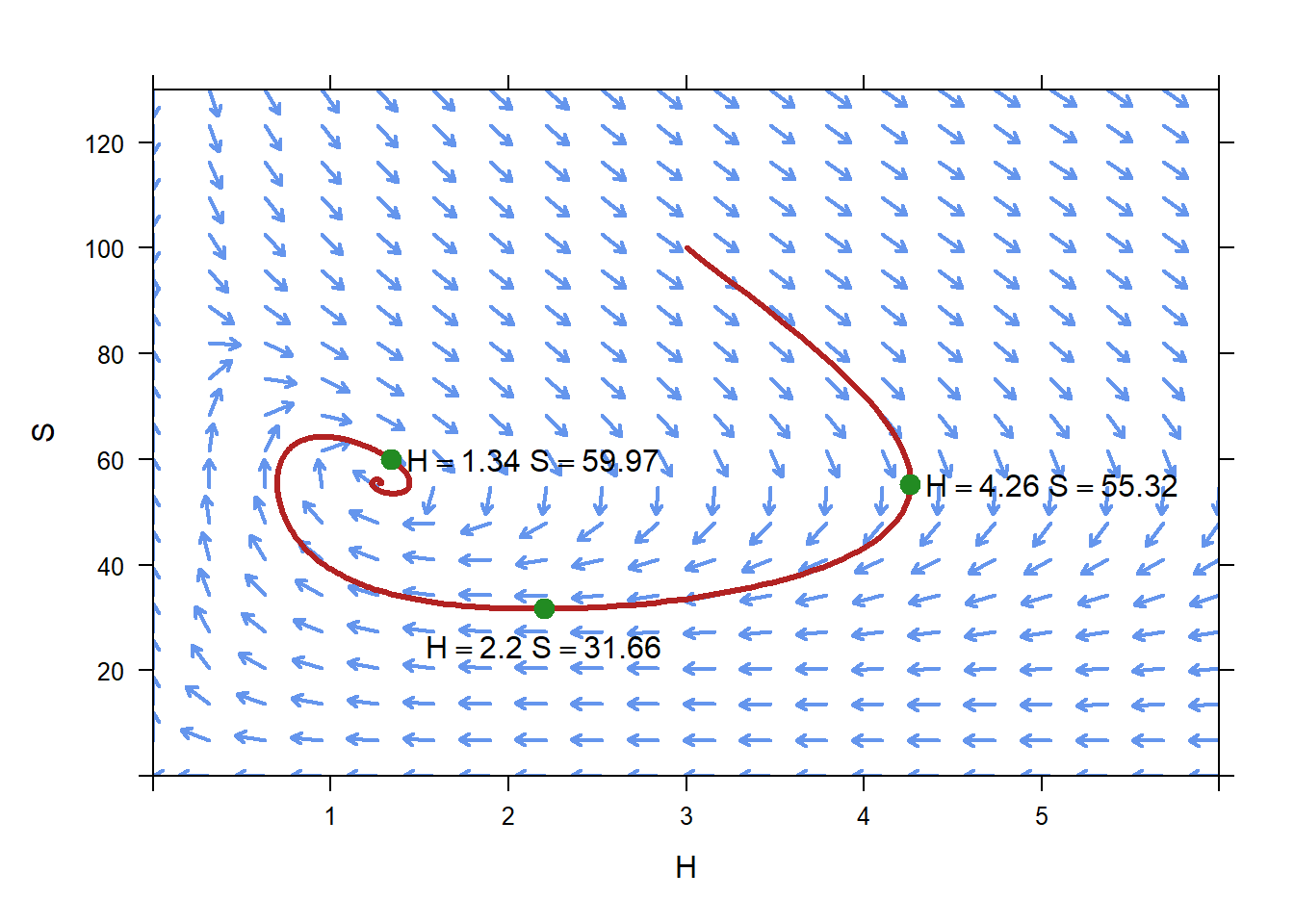
ics=c(H0,S0))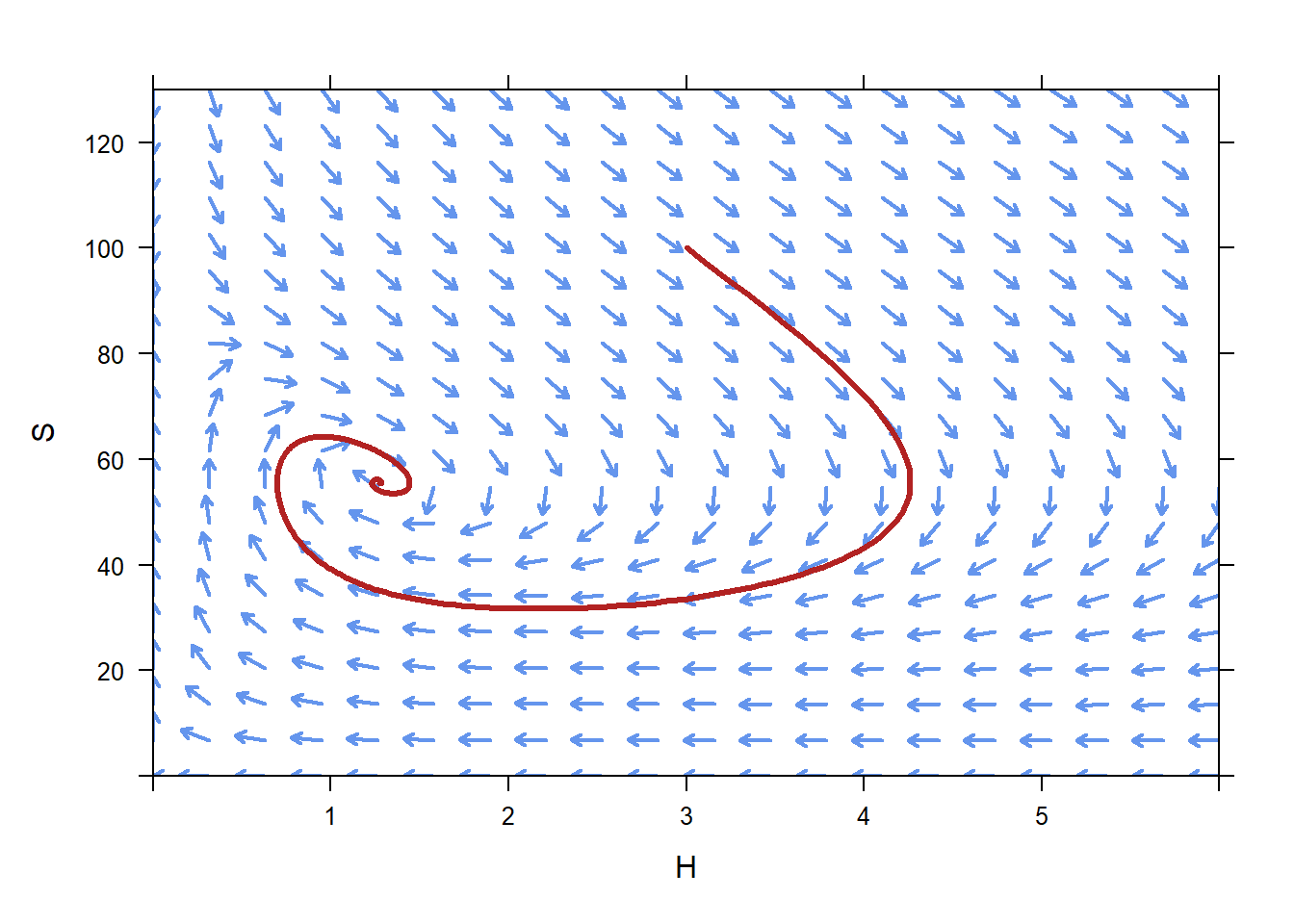 On this phase plane, we can see that if the population is initially \(H=3\), \(S=100\), then after a long time we expect that the population will be near \(H=1.2\), \(S=55\).
We need to be careful when we interpret a phase plane. Unlike a direction field, there is no time axis on a phase plane. When we plot a trajectory on a phase plane we can see what values we expect a population to take on from the given initial condition, but we can not immediately say at what time we expect the solution to take on those values. For instance, the point
(4.26,55.32) is on the trajectory. Therefore, we expect that if the initial population is \(H=3\), \(S=100\), we expect that at some time (but we don’t know what time from looking at this figure) the population will reach \(H=4.26\), \(S=55.32\).
Similarly, we expect that at some time the population will reach \(H=2.2\), \(S=31.66\), and
that even later the population will reach \(H=1.34\), \(S=59.97\).
10.4 Stability of Equilibrium Solutions
Let us return to Example 10.2.1.
\[\begin{aligned}
H'&=-0.5H+0.003SH\\
S'&=0.3S\left(1-\frac{S}{90}\right) - 0.03SH.
\end{aligned}\]
We saw that there are three equilibrium solutions for this system of IVPs.
## S H
## 1 0.000 0.000
## 2 55.556 1.276
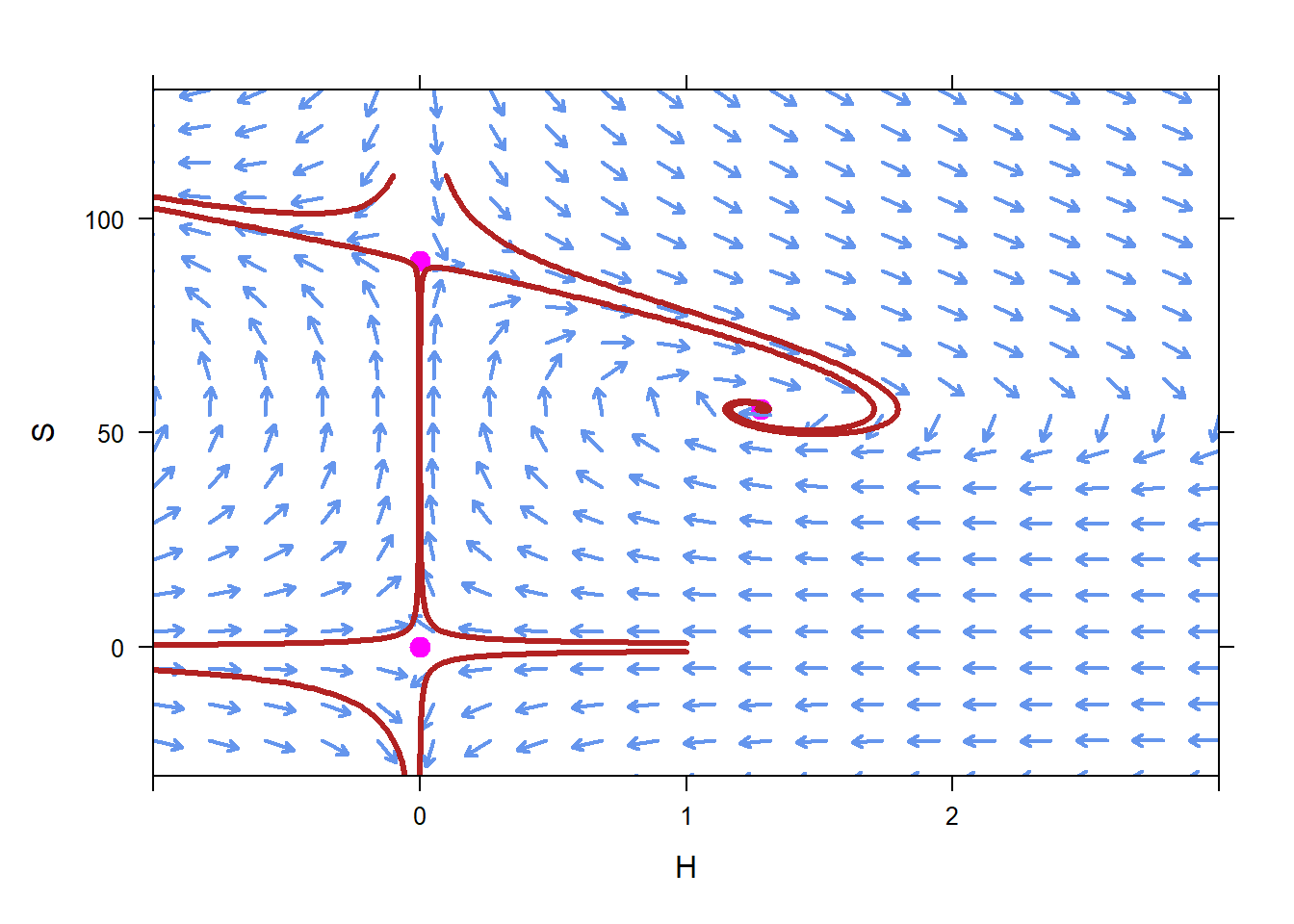
## 3 90.000 0.000We can draw a phase plane for this system of ODEs, making the axes large enough that we can see all of the equilibrium solutions. We also add a dot at each equilibrium solution; the dots are helpful for visualization but are not a part of this course.
plotPhasePlane(c(-0.5*H+0.009*S*H,0.3*S*(1-S/90)-0.09*S*H)~H&S,
               xlim=c(-1,3),ylim=c(-30,130))
plotPoints(c(0,55.55,90)~c(0,1.28,0),pch=19,cex=1.3,add=TRUE,col="magenta")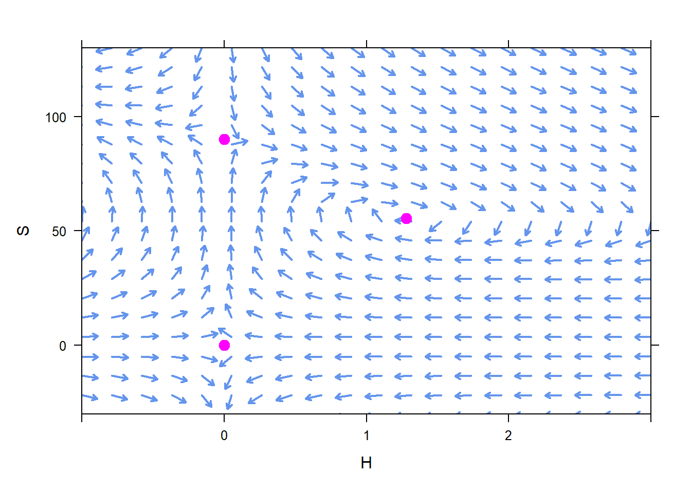
In examining the equilibrium solutions, we can see that initial conditions near \((H=1.3,S=55.6 )\) result in populations that oscillate, but ultimately stay near \((H=1.3,S=55.6)\). This makes \((H=1.3,S=55.6)\) a stable equilibrium solution. If we try plotting a few trajectories from nearby initial conditions, we see the trajectories heading toward the equilibrium solution.
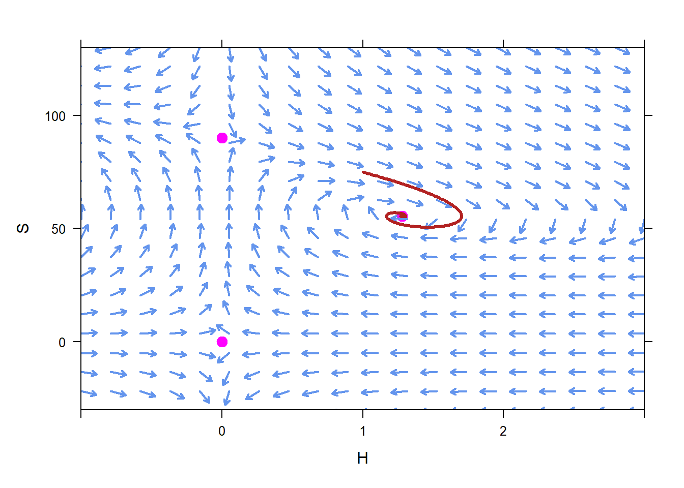
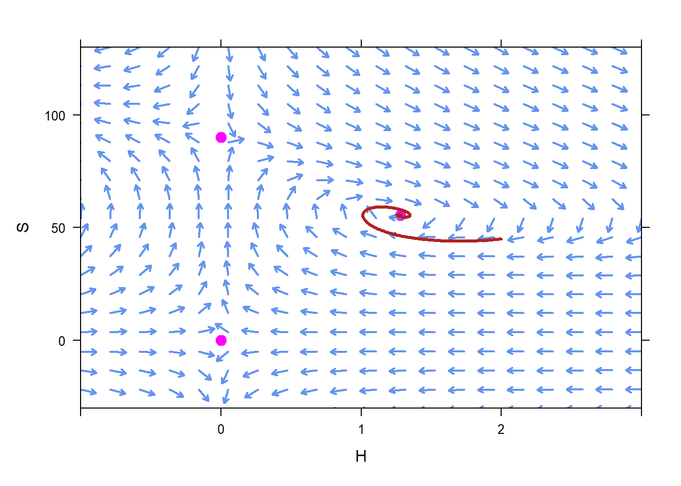
On the other hand, initial conditions near the other two equilibrium solutions, \(H=0\), \(S=0\) and \(H=0\), \(S=90\), lead to populations that tend away from those two equilibrium solutions. Therefore we call those equilibrium solutions unstable.
10.5 Examples
10.5.1 Competing Species
Consider a park in which squirrels(\(S\)) and rabbits (\(R\))live. Squirrels and rabbits compete for similar resources, but do not directly interact with each other. One set of equations for describing their population is \[\begin{aligned} S'&=0.006S(80-S-0.5R)\\ R'&=0.009R(95-P-1.1S). \end{aligned}\] First, we can identify all of the equilibrium solutions to this system of ODEs.
##        S      R
## 1  0.000  0.000
## 2  0.000 95.000
## 3 72.222 15.556
## 4 80.000  0.000
Next, we can plot a phase plane and add dots at the equilibrium solutions. We can then classify the stability of each equilibrium solution.
plotPhasePlane(c(0.006*S*(80-S-0.5*R),
0.009*R*(95-R-1.1*S))~S&R,xlim=c(-10,100),ylim=c(-10,110),N=30)
plotPoints(c(0,95,15.556,0)~c(0,0,72.222,80),col="magenta",pch=19,cex=1.3,add=TRUE)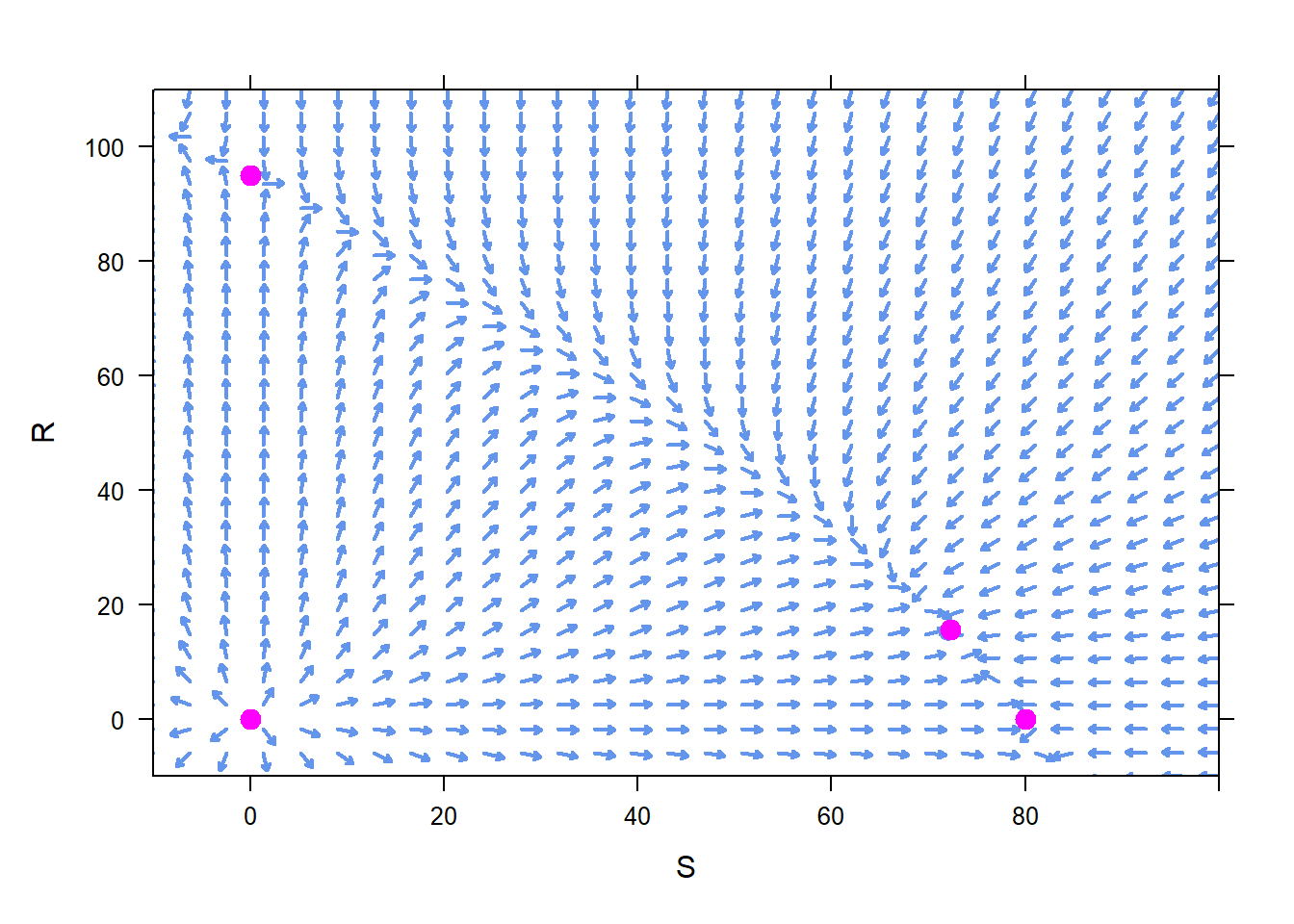 Just based on this figure, we are pretty sure that the equilibirum solution \(R=0\), \(S=0\) is unstable. Similarly, \(S=0\), \(R=95\) is unstable. Th other two are a little harder to determine, so we add a few trajectories starting nearby to help us determine the stability of each equilibrium solution.
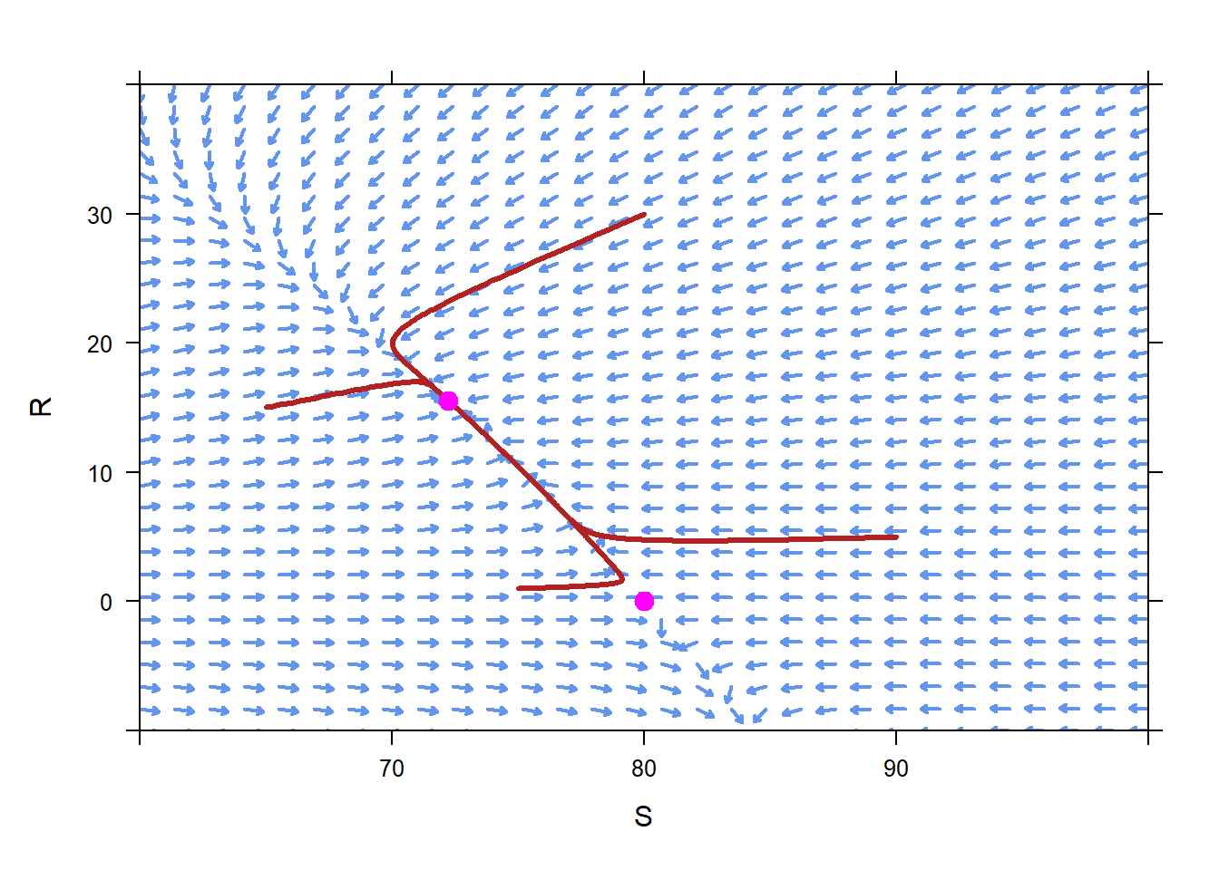 From this figure we can see that \(R=0\), \(S=80\) is an unstable equilibrium solution. We can also see that \(S=72.2\), \(H=15.6\) is a stable equilibrium solution.
10.5.1.1 Interpretation
We can interpret the fact that \(S=72.2\), \(R=15.6\) is a stable equilibrium solution as “if the population of squirrels and rabbits was exactly in balance, \(S=72.2\), \(R=15.6\), and suddenly one rabbit or one squirrel were removed fromt he population, the population would recover and tend back toward \(S=72.2\), \(H=R.6\)”. This is the notion of stability – small changes to the system will not impact the long-term behavior of the system.
On the other hand, consider the equilibrium solution at \(S=0\), \(R=0\). If we start with exactly 0 squirrels and exactly zero rabbits, then the two populations stay at 0. However, if the initial condition is even a tiny bit off of \(S=0\), \(R=0\), then in the long term the populations of rabbits and squirrels will be dramatically different from \(S=0\), \(R=0\).
The other two equilibrium solutions are also unstable. Even if the population is perfectly balanced, say at \(S=80\), \(R=0\), the addition of even one rabbit to the population will completely change the long-term term population away from \(S=80\), \(R=0\). This is the fundamental notion of instability – small changes to the system now compound and create very large future changes.
10.5.2 Lanchester’s Laws
Lanchester’s Laws were developed during World War I to describe battlefield dynamics, particularly in the context of trench warfare. Since then, multiple variations on Lanchester’s Laws have been developed to describe more complicated battlefield scenarios.
In their simplest form, Lanchester’s Laws describe the population of two forces, Blue and Red. Let \(B(t)\) be the number of soldiers currently fighting on the side of Blue, and \(R(t)\) the number of soldiers currently fighting on the side of Red.
The number of Red forces present on the battlefield changes due to attack from Blue forces. In particular, suppose that each Blue soldier can incapacitate \(\alpha\) Red soldiers/time. The, \[\frac{dR}{dt}=-\alpha B.\] If, similarly, each Red soldier can incapacitate \(\beta\) Blue soldier/time, then \[\frac{dB}{dt}=-\beta R.\] It could very well be that \(\alpha \neq \beta\) due to differences in weaponry, strategy, training, or fortifications. In this context, the coefficients \(\alpha\) and \(\beta\) are called the firepower coefficients.
Suppose that \(\alpha = 1.3\) hour-1, and that \(\beta = 1.0\) hour-1. Therefore, for some reason, Blue has the superior firepower.
First, we find the equilibrium solutions to the ODEs. This system is simple enough that we could easily solve by hand to find the only equilibrium solutions are \(A=0\), \(B=0\). Nevertheless, findZeros can also help us.
##   R B
## 1 0 0
Next we draw the phase plane.
plotPhasePlane(c(-1.3*B,-1.0*R)~R&B,xlim=c(-50,1000),ylim=c(-50,1000))
mathaxis.on()
plotPoints(c(0)~c(0),add=TRUE,pch=19,cex=1.3,col="magenta")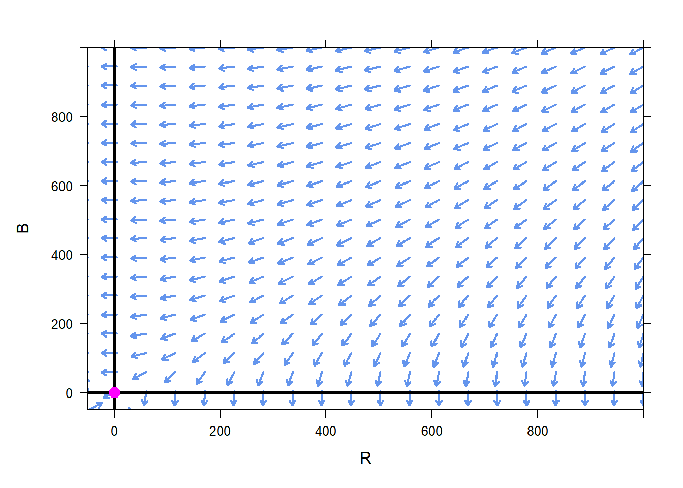 Now we can experiment with different initial conditions, that is, different initial numbers of soldiers, and see what the phase plane says about the outcome of the battle.
For instance, if initially \(R=600\) and \(B=700\), then we expect that the Blue army will win, since the trajectory originating at \((R=600,B=700)\) crosses the \(R=0\) axis. As a reminder, the phase plane does not tell us the time at which we get to the \(R=0\) state, it just tells that at some time we will get there. This is expected, since Blue had superior firepower and had superior initial numbers.
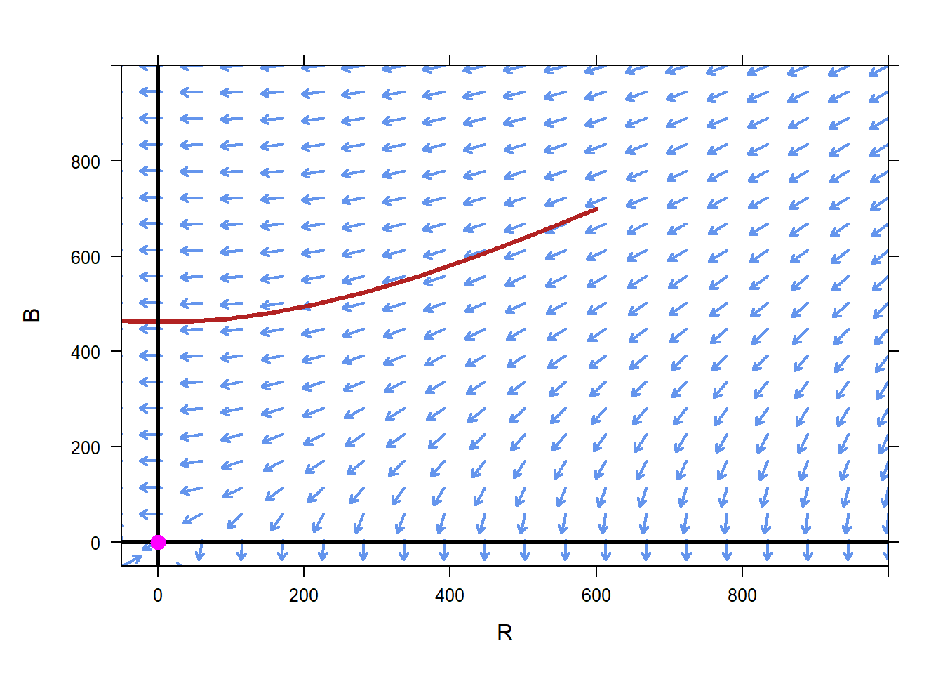
Interestingly, at the time the Red army is defeated, the equations predict that there will be over 400 Blue troops remaining. This is much greater than the initial difference between Red and Blue of 100 troops.
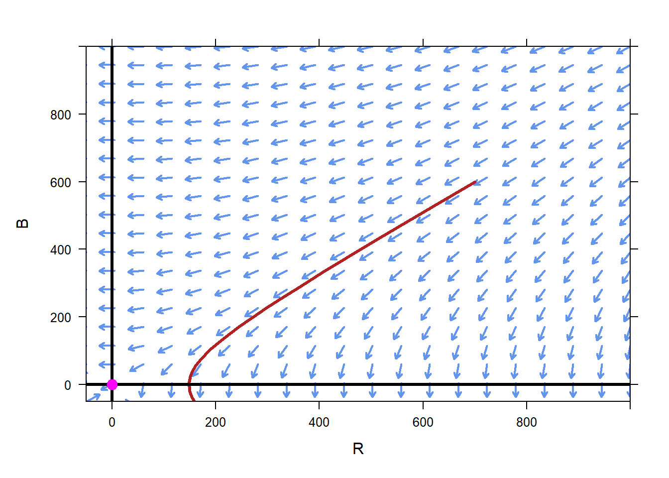
If the scenario were to change, and the Red army initially had 700 soldiers and the Blue army 600 soldiers, we can see that the phase plane tells us that the Red forces will win the battle, and will have a little less than 200 soldiers remaining when they do so.
 With the Lanchester model in hand, we can begin analyzing what-if scenarios. Suppose that we had estimated that the Blue forces numbered 750. What is the smallest Blue force that is predicted to prevail?
To answer the question, we can simply try several different initial conditions for \(B\), with a fixed initial condition for \(R\) of \(R=750\). Remembering that Blue has superior firepower, we expect that Blue can win the battle with fewer than 750 soldiers. A little experimentation shows that if initially \(B=658\), then Blue wins the battle.
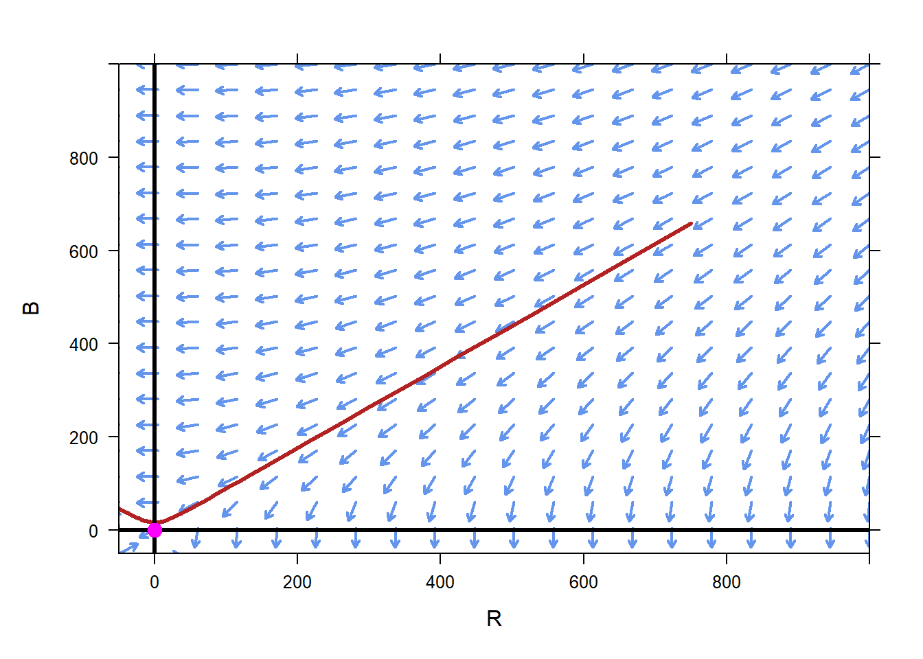 In this case, Blue wins the battle with barely any remaining soldiers. However, increasing the initial number of Blue soldiers to 668 from 658 means a much more decisive victory for Blue, with well over 100 soldiers remaining at the end of the battle. Such is the power of differential equations. Differential equations allow us to express relationships in a way we can easily interpret. The results that come out of the differential equations may well be counter intuitive, but because we believe in the underlying models, so to we must believe in the results.

10.5.3 Pendulum
Returning to Example 10.2.3, we have a pendulum with length 2 meters. \(x(t)\) is the angle between the pendulum and a vertical line passing through the pivot point, and \(y(t)\) is the angular velocity of the pendulum. The differential equations describing this motion are \[\begin{aligned} x'&=y\\ y'&=-4.9\sin(x). \end{aligned}\]
We can see that there are many equilibirium solutions for this system of ODEs
After some reflection, we see that the equilibrium solutions are at \(x=k\pi\), where \(k\) is an integer, and \(y=0\). That is, the pendulum will not move if it has zero angular velocity ,\(y=0\), and if it has position that is a multiple of \(\pi\). If \(x\) is an even multiple of \(\pi\), then the pendulum is hanging straight down. If \(x\) is an odd multiple of \(\pi\), then the pendulum is pointing straight up from the pivot point.
We can create a phase plane to ascertain the stability of the equilbrium solutions.
 Interestingly, the equilibrium solutions have very different behaviors. Initial conditions near even-multiple of \(\pi\) equilibrium solutions lead to trajectories that stay nearby the corresponding equilibrium solution.
That is, even-multiple of \(\pi\) equilibrium solutions are stable.
For example, physically, we know that if the initial condition is \(x=0\), \(y=0\), then we expect the pendulum to stay at \(x=0\), \(y=0\) forever, since the pendulum is starting at rest and hanging straight down from equilibrium. An animation of the corresponding motion is quite boring.
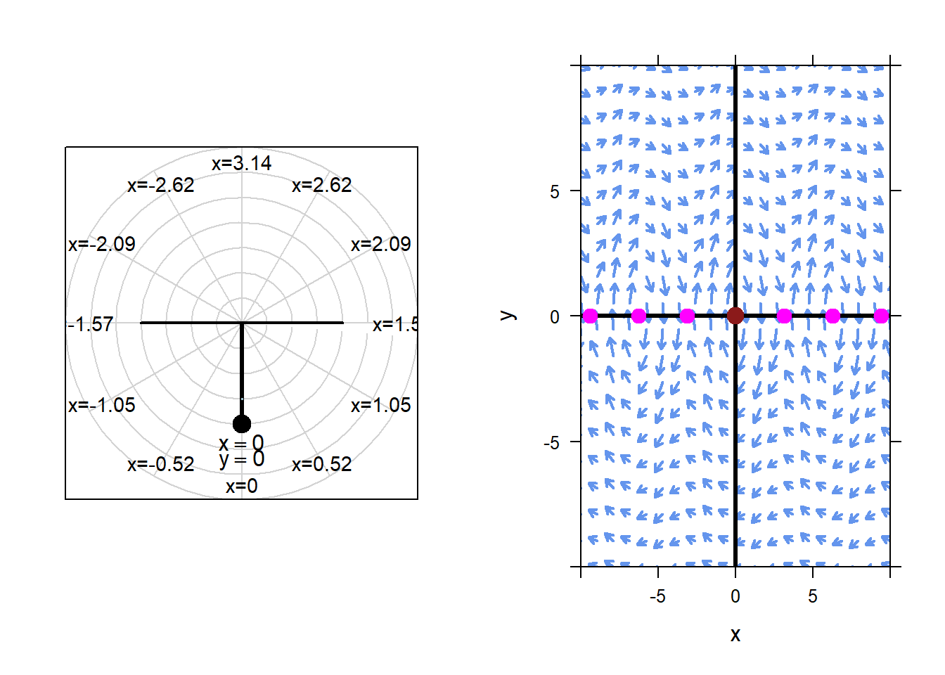
The figure above may look static, but it is in fact an animation of the motion of the pendulum if the initial condition is \(x=0\), \(y=0\). Since \(x=0\), \(y=0\) is an equilibrium solution, the animation is quite boring.
If we start the pendulum with an initial condition near \(x=0\), \(y=0\), the resulting motion stays similar to the equilibrium solution. For example, below is an animation with initial condition \(x=0.5\), \(y=0.1\).
Again, this is the nature of stability. Changing the initial conditions a little bit from the equilibrium initial conditions will not change the long term behavior of the system significantly.
The odd-multiple equilibrium solutions, however, are unstable. For example, consider the equilibrium solution at \(x=\pi\), \(y=0\). This corresponds to the pendulum being perfectly balanced upside down. From this initial configuration, the pendulum will never move.
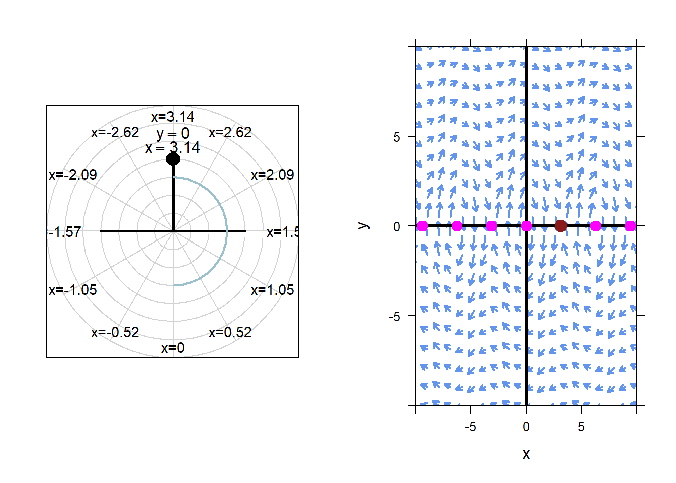
However, if we change the initial condition even a tiny bit, the pendulum will behave very differently than the equilibrium solution. For example, below we animate the results of initial condition \(x=\pi\), \(y=-0.1\).

This is the nature of unstable equilibrium solutions. Even tiny changes to the equilibrium initial conditions lead to dramatic changes to the resulting solution.
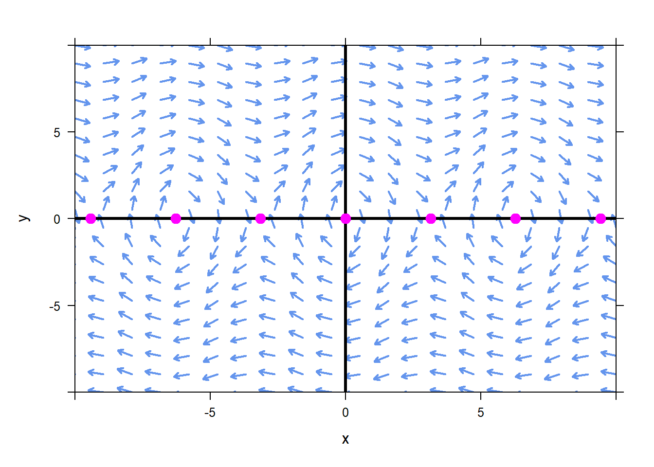
In the figure below we can see the very interesting phase plane for this system of ODEs, and the trajectories for a few different initial conditions.
plotPhasePlane(c(y,-4.9*sin(x))~x&y,xlim=c(-10,10),ylim=c(-10,10),ics=list(c(0,1.5),c(-3*pi,1.5),c(3*pi,-1.5),c(-2*pi,1.5),c(2*pi,1.5)))
mathaxis.on()
plotPoints(c(0,0,0,0,0,0,0)~c(-3*pi,-2*pi,-1*pi,0,pi,2*pi,3*pi),add=TRUE,pch=19,cex=1.3,col="magenta")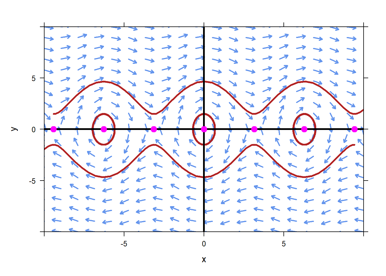
10.6 Exercises
Problems 1) – 3). Complete two steps per problem: a) Verify that the given solution satisfies the system of 1st order ODEs, and b) find the particular solution by solving for the constants, \(C_{1}\) and \(C_{2}\).
| System | Solution to the system | ICs | |
|---|---|---|---|
| 1) | \[\begin{aligned} u' &= 3u - 2v \\ v' &= 4u - 3v\ \end{aligned}\] | \[\begin{aligned} u &= C_{1}e^{- t} + C_{2}e^{t} \\ v &= 2C_{1}e^{- t} + C_{2}e^{t} \end{aligned}\] | \[\begin{aligned} u(0) &= - 2 \\ v(0) &= 1 \end{aligned}\] |
| 2) | \[\begin{aligned} p' &= - 3p + 3q \\ q' &= 2p - 2q\ \end{aligned}\] | \[\begin{aligned} p &= 3C_{1}e^{- 5t} + C_{2} \\ q &= -2C_{1}e^{- 5t} + C_{2} \end{aligned}\] | \[\begin{aligned} p(0) &= - 1 \\ q(0) &= 4 \end{aligned}\] |
| 3) | \[\begin{aligned} x' &= - x - 2y \\ y' &= x + y\ \end{aligned}\] | \[\begin{aligned} x &= C_{1}\cos(t) - (C_{1} + 2C_{2})\sin(t) \\ y &= C_{2}\cos(t) + (C_{1} + C_{2})\sin(t) \end{aligned}\] | \[\begin{aligned} x(0) &= - 1 \\ y(0) &= 2 \end{aligned}\] |
Problems 4) – 9). Find the equilibrium solution(s) for each system of 1st order ODEs. Classify each equilibrium solution as stable or unstable.
- \[\begin{aligned} y' &= - 3y + z \\ z' &= 2y - 5z\ \end{aligned}\]
- \[\begin{aligned} x' &= x - 1 \\ y' &= 2x + xy \end{aligned}\]
- \[\begin{aligned} u' &= - 3v + uv \\ v' &= 4u - 2uv \end{aligned}\]
- \[\begin{aligned} p' &= 6p + 0.1pq \\ q' &= - 12q + 0.4pq \end{aligned}\]
- \[\begin{aligned} r' &= r - rs \\ s' &= 2s(3 - s) - rs \end{aligned}\]
- \[\begin{aligned} x' &= y^{2} - y + 3xy \\ y' &= x^{2} + x\ \end{aligned}\]