plm Package
The plm package in R is designed for panel data analysis, allowing users to estimate various models, including pooled OLS, fixed effects, random effects, and other specifications commonly used in econometrics.
For a detailed guide, refer to:
# Load the package
library("plm")

data("Produc", package = "plm")

# Display first few rows
head(Produc)
#>     state year region     pcap     hwy   water    util       pc   gsp    emp
#> 1 ALABAMA 1970      6 15032.67 7325.80 1655.68 6051.20 35793.80 28418 1010.5
#> 2 ALABAMA 1971      6 15501.94 7525.94 1721.02 6254.98 37299.91 29375 1021.9
#> 3 ALABAMA 1972      6 15972.41 7765.42 1764.75 6442.23 38670.30 31303 1072.3
#> 4 ALABAMA 1973      6 16406.26 7907.66 1742.41 6756.19 40084.01 33430 1135.5
#> 5 ALABAMA 1974      6 16762.67 8025.52 1734.85 7002.29 42057.31 33749 1169.8
#> 6 ALABAMA 1975      6 17316.26 8158.23 1752.27 7405.76 43971.71 33604 1155.4
#>   unemp
#> 1   4.7
#> 2   5.2
#> 3   4.7
#> 4   3.9
#> 5   5.5
#> 6   7.7
To specify panel data, we define the individual (cross-sectional) and time identifiers:
# Convert data to panel format
pdata <- pdata.frame(Produc, index = c("state", "year"))

# Check structure
summary(pdata)
#>          state          year         region         pcap             hwy
#>  ALABAMA    : 17   1970   : 48   5      :136   Min.   :  2627   Min.   : 1827
#>  ARIZONA    : 17   1971   : 48   8      :136   1st Qu.:  7097   1st Qu.: 3858
#>  ARKANSAS   : 17   1972   : 48   4      :119   Median : 17572   Median : 7556
#>  CALIFORNIA : 17   1973   : 48   1      :102   Mean   : 25037   Mean   :10218
#>  COLORADO   : 17   1974   : 48   3      : 85   3rd Qu.: 27692   3rd Qu.:11267
#>  CONNECTICUT: 17   1975   : 48   6      : 68   Max.   :140217   Max.   :47699
#>  (Other)    :714   (Other):528   (Other):170
#>      water              util               pc              gsp
#>  Min.   :  228.5   Min.   :  538.5   Min.   :  4053   Min.   :  4354
#>  1st Qu.:  764.5   1st Qu.: 2488.3   1st Qu.: 21651   1st Qu.: 16503
#>  Median : 2266.5   Median : 7008.8   Median : 40671   Median : 39987
#>  Mean   : 3618.8   Mean   :11199.5   Mean   : 58188   Mean   : 61014
#>  3rd Qu.: 4318.7   3rd Qu.:11598.5   3rd Qu.: 64796   3rd Qu.: 68126
#>  Max.   :24592.3   Max.   :80728.1   Max.   :375342   Max.   :464550
#>
#>       emp              unemp
#>  Min.   :  108.3   Min.   : 2.800
#>  1st Qu.:  475.0   1st Qu.: 5.000
#>  Median : 1164.8   Median : 6.200
#>  Mean   : 1747.1   Mean   : 6.602
#>  3rd Qu.: 2114.1   3rd Qu.: 7.900
#>  Max.   :11258.0   Max.   :18.000
#>
The plm package allows for the estimation of several different panel data models.
- Pooled OLS Estimator
A simple pooled OLS model assumes a common intercept and ignores individual-specific effects.
pooling <- plm(log(gsp) ~ log(pcap) + log(emp) + unemp,
               data = pdata,
               model = "pooling")
summary(pooling)
#> Pooling Model
#>
#> Call:
#> plm(formula = log(gsp) ~ log(pcap) + log(emp) + unemp, data = pdata,
#>     model = "pooling")
#>
#> Balanced Panel: n = 48, T = 17, N = 816
#>
#> Residuals:
#>      Min.   1st Qu.    Median   3rd Qu.      Max.
#> -0.302260 -0.085204 -0.018166  0.051783  0.500144
#>
#> Coefficients:
#>               Estimate Std. Error t-value Pr(>|t|)
#> (Intercept)  2.2124123  0.0790988 27.9703  < 2e-16 ***
#> log(pcap)    0.4121307  0.0216314 19.0525  < 2e-16 ***
#> log(emp)     0.6205834  0.0199495 31.1078  < 2e-16 ***
#> unemp       -0.0035444  0.0020539 -1.7257  0.08478 .
#> ---
#> Signif. codes:  0 '***' 0.001 '**' 0.01 '*' 0.05 '.' 0.1 ' ' 1
#>
#> Total Sum of Squares:    849.81
#> Residual Sum of Squares: 13.326
#> R-Squared:      0.98432
#> Adj. R-Squared: 0.98426
#> F-statistic: 16990.2 on 3 and 812 DF, p-value: < 2.22e-16
- Between Estimator
This estimator takes the average over time for each entity, reducing within-group variation.
between <- plm(log(gsp) ~ log(pcap) + log(emp) + unemp,
               data = pdata, model = "between")
summary(between)
#> Oneway (individual) effect Between Model
#>
#> Call:
#> plm(formula = log(gsp) ~ log(pcap) + log(emp) + unemp, data = pdata,
#>     model = "between")
#>
#> Balanced Panel: n = 48, T = 17, N = 816
#> Observations used in estimation: 48
#>
#> Residuals:
#>      Min.   1st Qu.    Median   3rd Qu.      Max.
#> -0.172055 -0.086456 -0.013203  0.038100  0.394336
#>
#> Coefficients:
#>               Estimate Std. Error t-value  Pr(>|t|)
#> (Intercept)  2.0784403  0.3277756  6.3410 1.063e-07 ***
#> log(pcap)    0.4585009  0.0892620  5.1366 6.134e-06 ***
#> log(emp)     0.5751005  0.0828921  6.9379 1.410e-08 ***
#> unemp       -0.0031585  0.0145683 -0.2168    0.8294
#> ---
#> Signif. codes:  0 '***' 0.001 '**' 0.01 '*' 0.05 '.' 0.1 ' ' 1
#>
#> Total Sum of Squares:    48.875
#> Residual Sum of Squares: 0.65861
#> R-Squared:      0.98652
#> Adj. R-Squared: 0.98561
#> F-statistic: 1073.73 on 3 and 44 DF, p-value: < 2.22e-16
- First-Differences Estimator
The first-differences model eliminates time-invariant effects by differencing adjacent periods.
firstdiff <- plm(log(gsp) ~ log(pcap) + log(emp) + unemp,
                 data = pdata, model = "fd")
summary(firstdiff)
#> Oneway (individual) effect First-Difference Model
#>
#> Call:
#> plm(formula = log(gsp) ~ log(pcap) + log(emp) + unemp, data = pdata,
#>     model = "fd")
#>
#> Balanced Panel: n = 48, T = 17, N = 816
#> Observations used in estimation: 768
#>
#> Residuals:
#>       Min.    1st Qu.     Median    3rd Qu.       Max.
#> -0.0846921 -0.0108511  0.0016861  0.0124968  0.1018911
#>
#> Coefficients:
#>               Estimate Std. Error t-value  Pr(>|t|)
#> (Intercept)  0.0101353  0.0013206  7.6749 5.058e-14 ***
#> log(pcap)   -0.0167634  0.0453958 -0.3693     0.712
#> log(emp)     0.8212694  0.0362737 22.6409 < 2.2e-16 ***
#> unemp       -0.0061615  0.0007516 -8.1978 1.032e-15 ***
#> ---
#> Signif. codes:  0 '***' 0.001 '**' 0.01 '*' 0.05 '.' 0.1 ' ' 1
#>
#> Total Sum of Squares:    1.0802
#> Residual Sum of Squares: 0.33394
#> R-Squared:      0.69086
#> Adj. R-Squared: 0.68965
#> F-statistic: 569.123 on 3 and 764 DF, p-value: < 2.22e-16
- Fixed Effects (Within) Estimator
Controls for time-invariant heterogeneity by demeaning data within individuals.
fixed <- plm(log(gsp) ~ log(pcap) + log(emp) + unemp,
             data = pdata, model = "within")
summary(fixed)
#> Oneway (individual) effect Within Model
#>
#> Call:
#> plm(formula = log(gsp) ~ log(pcap) + log(emp) + unemp, data = pdata,
#>     model = "within")
#>
#> Balanced Panel: n = 48, T = 17, N = 816
#>
#> Residuals:
#>       Min.    1st Qu.     Median    3rd Qu.       Max.
#> -0.1253873 -0.0248746 -0.0054276  0.0184698  0.2026394
#>
#> Coefficients:
#>              Estimate  Std. Error t-value Pr(>|t|)
#> log(pcap)  0.03488447  0.03092191  1.1281   0.2596
#> log(emp)   1.03017988  0.02161353 47.6636   <2e-16 ***
#> unemp     -0.00021084  0.00096121 -0.2194   0.8264
#> ---
#> Signif. codes:  0 '***' 0.001 '**' 0.01 '*' 0.05 '.' 0.1 ' ' 1
#>
#> Total Sum of Squares:    18.941
#> Residual Sum of Squares: 1.3077
#> R-Squared:      0.93096
#> Adj. R-Squared: 0.92645
#> F-statistic: 3438.48 on 3 and 765 DF, p-value: < 2.22e-16
- Random Effects Estimator
Accounts for unobserved heterogeneity by modeling it as a random component.
random <- plm(log(gsp) ~ log(pcap) + log(emp) + unemp,
              data = pdata, model = "random")
summary(random)
#> Oneway (individual) effect Random Effect Model
#>    (Swamy-Arora's transformation)
#>
#> Call:
#> plm(formula = log(gsp) ~ log(pcap) + log(emp) + unemp, data = pdata,
#>     model = "random")
#>
#> Balanced Panel: n = 48, T = 17, N = 816
#>
#> Effects:
#>                    var  std.dev share
#> idiosyncratic 0.001709 0.041345 0.103
#> individual    0.014868 0.121934 0.897
#> theta: 0.918
#>
#> Residuals:
#>       Min.    1st Qu.     Median    3rd Qu.       Max.
#> -0.1246674 -0.0268273 -0.0049657  0.0214145  0.2389889
#>
#> Coefficients:
#>               Estimate Std. Error z-value Pr(>|z|)
#> (Intercept) 3.10569727 0.14715985 21.1042   <2e-16 ***
#> log(pcap)   0.03708054 0.02747015  1.3498   0.1771
#> log(emp)    1.00937552 0.02103951 47.9752   <2e-16 ***
#> unemp       0.00004806 0.00092301  0.0521   0.9585
#> ---
#> Signif. codes:  0 '***' 0.001 '**' 0.01 '*' 0.05 '.' 0.1 ' ' 1
#>
#> Total Sum of Squares:    24.523
#> Residual Sum of Squares: 1.4425
#> R-Squared:      0.94118
#> Adj. R-Squared: 0.94096
#> Chisq: 12992.5 on 3 DF, p-value: < 2.22e-16
Model Selection and Diagnostic Tests
- Lagrange Multiplier Test for Random Effects
The Breusch-Pagan LM test compares random effects with pooled OLS.
plmtest(pooling, effect = "individual", type = "bp")
#>
#>  Lagrange Multiplier Test - (Breusch-Pagan)
#>
#> data:  log(gsp) ~ log(pcap) + log(emp) + unemp
#> chisq = 4567.1, df = 1, p-value < 2.2e-16
#> alternative hypothesis: significant effects
Other test types: "honda", "kw", "ghm". Other effects: "time", "twoways".
- Cross-Sectional Dependence Tests
Breusch-Pagan LM test for cross-sectional dependence
pcdtest(fixed, test = "lm")
#>
#>  Breusch-Pagan LM test for cross-sectional dependence in panels
#>
#> data:  log(gsp) ~ log(pcap) + log(emp) + unemp
#> chisq = 6490.4, df = 1128, p-value < 2.2e-16
#> alternative hypothesis: cross-sectional dependence
Pesaran’s CD statistic
pcdtest(fixed, test = "cd")
#>
#>  Pesaran CD test for cross-sectional dependence in panels
#>
#> data:  log(gsp) ~ log(pcap) + log(emp) + unemp
#> z = 37.13, p-value < 2.2e-16
#> alternative hypothesis: cross-sectional dependence
- Serial Correlation Test (Panel Version of the Breusch-Godfrey Test)
Used to check for autocorrelation in panel data.
pbgtest(fixed)
#>
#>  Breusch-Godfrey/Wooldridge test for serial correlation in panel models
#>
#> data:  log(gsp) ~ log(pcap) + log(emp) + unemp
#> chisq = 476.92, df = 17, p-value < 2.2e-16
#> alternative hypothesis: serial correlation in idiosyncratic errors
- Stationarity Test (Augmented Dickey-Fuller Test)
Checks whether a time series variable is stationary.
library(tseries)
adf.test(pdata$gsp, k = 2)
#>
#>  Augmented Dickey-Fuller Test
#>
#> data:  pdata$gsp
#> Dickey-Fuller = -5.9028, Lag order = 2, p-value = 0.01
#> alternative hypothesis: stationary
- F-Test for Fixed Effects vs. Pooled OLS
pFtest(fixed, pooling)
#>
#>  F test for individual effects
#>
#> data:  log(gsp) ~ log(pcap) + log(emp) + unemp
#> F = 149.58, df1 = 47, df2 = 765, p-value < 2.2e-16
#> alternative hypothesis: significant effects
- Hausman Test for Fixed vs. Random Effects
phtest(random, fixed)
#>
#>  Hausman Test
#>
#> data:  log(gsp) ~ log(pcap) + log(emp) + unemp
#> chisq = 84.924, df = 3, p-value < 2.2e-16
#> alternative hypothesis: one model is inconsistent
Heteroskedasticity and Robust Standard Errors
- Breusch-Pagan Test for Heteroskedasticity
Tests whether heteroskedasticity is present in the panel dataset.
library(lmtest)
bptest(log(gsp) ~ log(pcap) + log(emp) + unemp,  data = pdata)
#>
#>  studentized Breusch-Pagan test
#>
#> data:  log(gsp) ~ log(pcap) + log(emp) + unemp
#> BP = 98.223, df = 3, p-value < 2.2e-16
- Correcting for Heteroskedasticity
If heteroskedasticity is detected, use robust standard errors:
For Random Effects Model
# Original coefficients
coeftest(random)
#>
#> t test of coefficients:
#>
#>               Estimate Std. Error t value Pr(>|t|)
#> (Intercept) 3.10569727 0.14715985 21.1042   <2e-16 ***
#> log(pcap)   0.03708054 0.02747015  1.3498   0.1774
#> log(emp)    1.00937552 0.02103951 47.9752   <2e-16 ***
#> unemp       0.00004806 0.00092301  0.0521   0.9585
#> ---
#> Signif. codes:  0 '***' 0.001 '**' 0.01 '*' 0.05 '.' 0.1 ' ' 1

# Heteroskedasticity-consistent standard errors
coeftest(random, vcovHC)
#>
#> t test of coefficients:
#>
#>               Estimate Std. Error t value Pr(>|t|)
#> (Intercept) 3.10569727 0.23261788 13.3511   <2e-16 ***
#> log(pcap)   0.03708054 0.06125725  0.6053   0.5451
#> log(emp)    1.00937552 0.06395880 15.7817   <2e-16 ***
#> unemp       0.00004806 0.00215219  0.0223   0.9822
#> ---
#> Signif. codes:  0 '***' 0.001 '**' 0.01 '*' 0.05 '.' 0.1 ' ' 1

# Different HC types
t(sapply(c("HC0", "HC1", "HC2", "HC3", "HC4"), function(x)
    sqrt(diag(vcovHC(random, type = x)))
))
#>     (Intercept)  log(pcap)   log(emp)       unemp
#> HC0   0.2326179 0.06125725 0.06395880 0.002152189
#> HC1   0.2331901 0.06140795 0.06411614 0.002157484
#> HC2   0.2334857 0.06161618 0.06439057 0.002160392
#> HC3   0.2343595 0.06197939 0.06482756 0.002168646
#> HC4   0.2342815 0.06235576 0.06537813 0.002168867
HC0: Default heteroskedasticity-consistent (White’s estimator).
HC1, HC2, HC3: Recommended for small samples.
HC4: Useful for small samples with influential observations.
For Fixed Effects Model
# Original coefficients
coeftest(fixed)
#>
#> t test of coefficients:
#>
#>              Estimate  Std. Error t value Pr(>|t|)
#> log(pcap)  0.03488447  0.03092191  1.1281   0.2596
#> log(emp)   1.03017988  0.02161353 47.6636   <2e-16 ***
#> unemp     -0.00021084  0.00096121 -0.2194   0.8264
#> ---
#> Signif. codes:  0 '***' 0.001 '**' 0.01 '*' 0.05 '.' 0.1 ' ' 1

# Heteroskedasticity-consistent standard errors
coeftest(fixed, vcovHC)
#>
#> t test of coefficients:
#>
#>              Estimate  Std. Error t value Pr(>|t|)
#> log(pcap)  0.03488447  0.06661083  0.5237   0.6006
#> log(emp)   1.03017988  0.06413365 16.0630   <2e-16 ***
#> unemp     -0.00021084  0.00217453 -0.0970   0.9228
#> ---
#> Signif. codes:  0 '***' 0.001 '**' 0.01 '*' 0.05 '.' 0.1 ' ' 1

# Arellano method for robust errors
coeftest(fixed, vcovHC(fixed, method = "arellano"))
#>
#> t test of coefficients:
#>
#>              Estimate  Std. Error t value Pr(>|t|)
#> log(pcap)  0.03488447  0.06661083  0.5237   0.6006
#> log(emp)   1.03017988  0.06413365 16.0630   <2e-16 ***
#> unemp     -0.00021084  0.00217453 -0.0970   0.9228
#> ---
#> Signif. codes:  0 '***' 0.001 '**' 0.01 '*' 0.05 '.' 0.1 ' ' 1

# Different HC types
t(sapply(c("HC0", "HC1", "HC2", "HC3", "HC4"), function(x)
    sqrt(diag(vcovHC(fixed, type = x)))
))
#>      log(pcap)   log(emp)       unemp
#> HC0 0.06661083 0.06413365 0.002174525
#> HC1 0.06673362 0.06425187 0.002178534
#> HC2 0.06689078 0.06441024 0.002182114
#> HC3 0.06717278 0.06468886 0.002189747
#> HC4 0.06742431 0.06496436 0.002193150
Summary of Model Selection
| LM Test |
OLS is appropriate |
Reject H₀ → Use RE |
| Hausman Test |
Random effects preferred |
Reject H₀ → Use FE |
| pFtest |
OLS is appropriate |
Reject H₀ → Use FE |
| Breusch-Pagan |
No heteroskedasticity |
Reject H₀ → Use robust SE |
Variance Components Structure
Beyond the standard random effects model, the plm package provides additional methods for estimating variance components models and instrumental variable techniques for dealing with endogeneity in panel data.
Different estimators for the variance components structure exist in the literature, and plm allows users to specify them through the random.method argument.
Random Effects Estimators:
Effects in Panel Models:
Individual effects (default).
Time effects (effect = "time").
Two-way effects (effect = "twoways").
amemiya <- plm(
    log(gsp) ~ log(pcap) + log(emp) + unemp,
    data = pdata,
    model = "random",
    random.method = "amemiya",
    effect = "twoways"
)

summary(amemiya)
#> Twoways effects Random Effect Model
#>    (Amemiya's transformation)
#>
#> Call:
#> plm(formula = log(gsp) ~ log(pcap) + log(emp) + unemp, data = pdata,
#>     effect = "twoways", model = "random", random.method = "amemiya")
#>
#> Balanced Panel: n = 48, T = 17, N = 816
#>
#> Effects:
#>                    var  std.dev share
#> idiosyncratic 0.001228 0.035039 0.028
#> individual    0.041201 0.202981 0.941
#> time          0.001359 0.036859 0.031
#> theta: 0.9582 (id) 0.8641 (time) 0.8622 (total)
#>
#> Residuals:
#>        Min.     1st Qu.      Median     3rd Qu.        Max.
#> -0.13796209 -0.01951506 -0.00053384  0.01807398  0.20452581
#>
#> Coefficients:
#>               Estimate Std. Error z-value  Pr(>|z|)
#> (Intercept)  3.9581876  0.1767036 22.4001 < 2.2e-16 ***
#> log(pcap)    0.0378443  0.0253963  1.4902  0.136184
#> log(emp)     0.8891887  0.0227677 39.0548 < 2.2e-16 ***
#> unemp       -0.0031568  0.0011240 -2.8086  0.004976 **
#> ---
#> Signif. codes:  0 '***' 0.001 '**' 0.01 '*' 0.05 '.' 0.1 ' ' 1
#>
#> Total Sum of Squares:    5.3265
#> Residual Sum of Squares: 0.98398
#> R-Squared:      0.81527
#> Adj. R-Squared: 0.81458
#> Chisq: 3583.53 on 3 DF, p-value: < 2.22e-16
The ercomp() function retrieves estimates of the variance components in a random effects model. Below, we extract the variance decomposition using Amemiya’s method:
ercomp(log(gsp) ~ log(pcap) + log(emp) + unemp,
       data = pdata,
       method = "amemiya",
       effect = "twoways")
#>                    var  std.dev share
#> idiosyncratic 0.001228 0.035039 0.028
#> individual    0.041201 0.202981 0.941
#> time          0.001359 0.036859 0.031
#> theta: 0.9582 (id) 0.8641 (time) 0.8622 (total)
This output includes:
Variance of the individual effect.
Variance of the time effect (if applicable).
Variance of the idiosyncratic error.
Checking Panel Data Balance
Panel datasets may be balanced (each individual has observations for all time periods) or unbalanced (some individuals are missing observations). The punbalancedness() function measures the degree of balance in the data, with values closer to 1 indicating a balanced panel (Ahrens and Pincus 1981).
Instrumental Variables in Panel Data
Instrumental variables (IV) are used to address endogeneity, which arises when regressors are correlated with the error term. plm provides various IV estimation methods through the inst.method argument.
Instrumental Variable Estimators
Other Estimators in Panel Data Models
Beyond standard fixed effects and random effects models, the plm package provides additional estimation techniques tailored for heterogeneous coefficients, dynamic panel models, and feasible generalized least squares (FGLS) methods.
Variable Coefficients Model (pvcm)
The variable coefficients model (VCM) allows coefficients to vary across cross-sectional units, accounting for unobserved heterogeneity more flexibly.
Two Estimation Approaches:
fixed_pvcm  <-
    pvcm(log(gsp) ~ log(pcap) + log(emp) + unemp,
         data = pdata,
         model = "within")
random_pvcm <-
    pvcm(log(gsp) ~ log(pcap) + log(emp) + unemp,
         data = pdata,
         model = "random")

summary(fixed_pvcm)
#> Oneway (individual) effect No-pooling model
#>
#> Call:
#> pvcm(formula = log(gsp) ~ log(pcap) + log(emp) + unemp, data = pdata,
#>     model = "within")
#>
#> Balanced Panel: n = 48, T = 17, N = 816
#>
#> Residuals:
#>         Min.      1st Qu.       Median      3rd Qu.         Max.
#> -0.075247625 -0.013247956  0.000666934  0.013852996  0.118966807
#>
#> Coefficients:
#>   (Intercept)        log(pcap)           log(emp)          unemp
#>  Min.   :-3.8868   Min.   :-1.11962   Min.   :0.3790   Min.   :-1.597e-02
#>  1st Qu.: 0.9917   1st Qu.:-0.38475   1st Qu.:0.8197   1st Qu.:-5.319e-03
#>  Median : 2.9848   Median :-0.03147   Median :1.1506   Median : 5.335e-05
#>  Mean   : 2.8079   Mean   :-0.06028   Mean   :1.1656   Mean   : 9.024e-04
#>  3rd Qu.: 4.3553   3rd Qu.: 0.25573   3rd Qu.:1.3779   3rd Qu.: 8.374e-03
#>  Max.   :12.8800   Max.   : 1.16922   Max.   :2.4276   Max.   : 2.507e-02
#>
#> Total Sum of Squares: 15729
#> Residual Sum of Squares: 0.40484
#> Multiple R-Squared: 0.99997
summary(random_pvcm)
#> Oneway (individual) effect Random coefficients model
#>
#> Call:
#> pvcm(formula = log(gsp) ~ log(pcap) + log(emp) + unemp, data = pdata,
#>     model = "random")
#>
#> Balanced Panel: n = 48, T = 17, N = 816
#>
#> Residuals:
#>     Min.  1st Qu.   Median     Mean  3rd Qu.     Max.
#> -0.23364 -0.03401  0.05558  0.09811  0.19349  1.14326
#>
#> Estimated mean of the coefficients:
#>                Estimate  Std. Error z-value  Pr(>|z|)
#> (Intercept)  2.79030044  0.53104167  5.2544 1.485e-07 ***
#> log(pcap)   -0.04195768  0.08621579 -0.4867    0.6265
#> log(emp)     1.14988911  0.07225221 15.9149 < 2.2e-16 ***
#> unemp        0.00031135  0.00163864  0.1900    0.8493
#> ---
#> Signif. codes:  0 '***' 0.001 '**' 0.01 '*' 0.05 '.' 0.1 ' ' 1
#>
#> Estimated variance of the coefficients:
#>             (Intercept) log(pcap)   log(emp)       unemp
#> (Intercept)  11.2648882 -1.335932  0.2035824  0.00827707
#> log(pcap)    -1.3359322  0.287021 -0.1872915 -0.00345298
#> log(emp)      0.2035824 -0.187291  0.2134845  0.00336374
#> unemp         0.0082771 -0.003453  0.0033637  0.00009425
#>
#> Total Sum of Squares: 15729
#> Residual Sum of Squares: 40.789
#> Multiple R-Squared: 0.99741
#> Chisq: 739.334 on 3 DF, p-value: < 2.22e-16
#> Test for parameter homogeneity: Chisq = 21768.8 on 188 DF, p-value: < 2.22e-16
Generalized Method of Moments Estimator (pgmm)
The Generalized Method of Moments estimator is commonly used for dynamic panel models, especially when:
library(plm)

# estimates a dynamic labor demand function using one-step GMM,
# applying lagged variables as instruments
z2 <- pgmm(
    log(emp) ~ lag(log(emp), 1) + lag(log(wage), 0:1) +
        lag(log(capital), 0:1) |
        lag(log(emp), 2:99) +
        lag(log(wage), 2:99) + lag(log(capital), 2:99),
    data = EmplUK,
    effect = "twoways",
    model = "onestep",
    transformation = "ld"
)

summary(z2, robust = TRUE)
#> Twoways effects One-step model System GMM
#>
#> Call:
#> pgmm(formula = log(emp) ~ lag(log(emp), 1) + lag(log(wage), 0:1) +
#>     lag(log(capital), 0:1) | lag(log(emp), 2:99) + lag(log(wage),
#>     2:99) + lag(log(capital), 2:99), data = EmplUK, effect = "twoways",
#>     model = "onestep", transformation = "ld")
#>
#> Unbalanced Panel: n = 140, T = 7-9, N = 1031
#>
#> Number of Observations Used: 1642
#> Residuals:
#>       Min.    1st Qu.     Median       Mean    3rd Qu.       Max.
#> -0.7530341 -0.0369030  0.0000000  0.0002882  0.0466069  0.6001503
#>
#> Coefficients:
#>                          Estimate Std. Error z-value  Pr(>|z|)
#> lag(log(emp), 1)         0.935605   0.026295 35.5810 < 2.2e-16 ***
#> lag(log(wage), 0:1)0    -0.630976   0.118054 -5.3448 9.050e-08 ***
#> lag(log(wage), 0:1)1     0.482620   0.136887  3.5257 0.0004224 ***
#> lag(log(capital), 0:1)0  0.483930   0.053867  8.9838 < 2.2e-16 ***
#> lag(log(capital), 0:1)1 -0.424393   0.058479 -7.2572 3.952e-13 ***
#> ---
#> Signif. codes:  0 '***' 0.001 '**' 0.01 '*' 0.05 '.' 0.1 ' ' 1
#>
#> Sargan test: chisq(100) = 118.763 (p-value = 0.097096)
#> Autocorrelation test (1): normal = -4.808434 (p-value = 1.5212e-06)
#> Autocorrelation test (2): normal = -0.2800133 (p-value = 0.77947)
#> Wald test for coefficients: chisq(5) = 11174.82 (p-value = < 2.22e-16)
#> Wald test for time dummies: chisq(7) = 14.71138 (p-value = 0.039882)
Explanation of Arguments:
log(emp) ~ lag(log(emp), 1) + lag(log(wage), 0:1) + lag(log(capital), 0:1)
→ Specifies the dynamic model, where log(emp) depends on its first lag and contemporaneous plus lagged values of log(wage) and log(capital).
| lag(log(emp), 2:99) + lag(log(wage), 2:99) + lag(log(capital), 2:99)
→ Instruments for endogenous regressors, using further lags.
effect = "twoways"
→ Includes both individual and time effects.
model = "onestep"
→ Uses one-step GMM (alternative: "twostep" for efficiency gain).
transformation = "ld"
→ Uses lagged differences as transformation.
Generalized Feasible Generalized Least Squares Models (pggls)
The FGLS estimator (pggls) is robust against:
However, it assumes no cross-sectional correlation and is most suitable when NNN (cross-sectional units) is much larger than TTT (time periods), i.e., long panels.
Random Effects FGLS Model:
zz <- pggls(
    log(emp) ~ log(wage) + log(capital),
    data = EmplUK,
    model = "pooling"
)

summary(zz)
#> Oneway (individual) effect General FGLS model
#>
#> Call:
#> pggls(formula = log(emp) ~ log(wage) + log(capital), data = EmplUK,
#>     model = "pooling")
#>
#> Unbalanced Panel: n = 140, T = 7-9, N = 1031
#>
#> Residuals:
#>     Min.  1st Qu.   Median     Mean  3rd Qu.     Max.
#> -1.80696 -0.36552  0.06181  0.03230  0.44279  1.58719
#>
#> Coefficients:
#>               Estimate Std. Error z-value  Pr(>|z|)
#> (Intercept)   2.023480   0.158468 12.7690 < 2.2e-16 ***
#> log(wage)    -0.232329   0.048001 -4.8401 1.298e-06 ***
#> log(capital)  0.610484   0.017434 35.0174 < 2.2e-16 ***
#> ---
#> Signif. codes:  0 '***' 0.001 '**' 0.01 '*' 0.05 '.' 0.1 ' ' 1
#> Total Sum of Squares: 1853.6
#> Residual Sum of Squares: 402.55
#> Multiple R-squared: 0.78283
Fixed Effects FGLS Model:
zz <- pggls(
    log(emp) ~ log(wage) + log(capital),
    data = EmplUK,
    model = "within"
)

summary(zz)
#> Oneway (individual) effect Within FGLS model
#>
#> Call:
#> pggls(formula = log(emp) ~ log(wage) + log(capital), data = EmplUK,
#>     model = "within")
#>
#> Unbalanced Panel: n = 140, T = 7-9, N = 1031
#>
#> Residuals:
#>         Min.      1st Qu.       Median      3rd Qu.         Max.
#> -0.508362414 -0.074254395 -0.002442181  0.076139063  0.601442300
#>
#> Coefficients:
#>               Estimate Std. Error z-value  Pr(>|z|)
#> log(wage)    -0.617617   0.030794 -20.056 < 2.2e-16 ***
#> log(capital)  0.561049   0.017185  32.648 < 2.2e-16 ***
#> ---
#> Signif. codes:  0 '***' 0.001 '**' 0.01 '*' 0.05 '.' 0.1 ' ' 1
#> Total Sum of Squares: 1853.6
#> Residual Sum of Squares: 17.368
#> Multiple R-squared: 0.99063
Key Considerations:
Efficient under the assumption of homoskedasticity.
Inefficient if there is group-wise heteroskedasticity.
Ideal for large-N, small-T panels.
Summary of Alternative Panel Data Estimators
Variable Coefficients (pvcm) |
Fixed (within), Random (random) |
Allows coefficients to vary across individuals. |
GMM (pgmm) |
One-step, Two-step |
Used in dynamic models with endogeneity. |
Feasible GLS (pggls) |
Fixed (within), Random (pooling) |
Handles heteroskedasticity and serial correlation but assumes no cross-sectional correlation. |
fixest Package
The fixest package provides efficient and flexible methods for estimating fixed effects and generalized linear models in panel data. It is optimized for handling large datasets with high-dimensional fixed effects and allows for multiple model estimation, robust standard errors, and split-sample estimation.
For further details, refer to the official fixest vignette.
Available Estimation Functions in fixest
feols |
Fixed effects OLS (linear regression) |
feglm |
Generalized linear models (GLMs) |
femlm |
Maximum likelihood estimation (MLE) |
feNmlm |
Non-linear models (non-linear in RHS parameters) |
fepois |
Poisson fixed-effects regression |
fenegbin |
Negative binomial fixed-effects regression |
Note: These functions work only for fixest objects.
library(fixest)
data(airquality)
# Setting a variable dictionary for output labeling
setFixest_dict(
c(
Ozone = "Ozone (ppb)",
Solar.R = "Solar Radiation (Langleys)",
Wind = "Wind Speed (mph)",
Temp = "Temperature"
)
)
# Fixed effects OLS with stepwise estimation and clustering
est <- feols(
Ozone ~ Solar.R + sw0(Wind + Temp) | csw(Month, Day),
data = airquality,
cluster = ~ Day
)
# Display results
etable(est)
#> est.1 est.2
#> Dependent Var.: Ozone (ppb) Ozone (ppb)
#>
#> Solar Radiation (Langleys) 0.1148*** (0.0234) 0.0522* (0.0202)
#> Wind Speed (mph) -3.109*** (0.7986)
#> Temperature 1.875*** (0.3671)
#> Fixed-Effects: ------------------ ------------------
#> Month Yes Yes
#> Day No No
#> __________________________ __________________ __________________
#> S.E.: Clustered by: Day by: Day
#> Observations 111 111
#> R2 0.31974 0.63686
#> Within R2 0.12245 0.53154
#>
#> est.3 est.4
#> Dependent Var.: Ozone (ppb) Ozone (ppb)
#>
#> Solar Radiation (Langleys) 0.1078** (0.0329) 0.0509* (0.0236)
#> Wind Speed (mph) -3.289*** (0.7777)
#> Temperature 2.052*** (0.2415)
#> Fixed-Effects: ----------------- ------------------
#> Month Yes Yes
#> Day Yes Yes
#> __________________________ _________________ __________________
#> S.E.: Clustered by: Day by: Day
#> Observations 111 111
#> R2 0.58018 0.81604
#> Within R2 0.12074 0.61471
#> ---
#> Signif. codes: 0 '***' 0.001 '**' 0.01 '*' 0.05 '.' 0.1 ' ' 1
# Output in LaTeX format
# etable(est, tex = TRUE)
# Extract fixed-effects coefficients
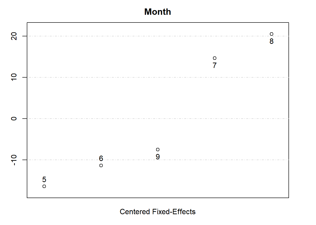
fixedEffects <- fixef(est[[1]])
summary(fixedEffects)
#> Fixed_effects coefficients
#> Number of fixed-effects for variable Month is 5.
#> Mean = 19.6 Variance = 272
#>
#> COEFFICIENTS:
#> Month: 5 6 7 8 9
#> 3.219 8.288 34.26 40.12 12.13
# View fixed effects for one dimension
fixedEffects$Month
#> 5 6 7 8 9
#> 3.218876 8.287899 34.260812 40.122257 12.130971
# Plot fixed effects
plot(fixedEffects)
This example demonstrates:
Fixed effects estimation (| csw(Month, Day)).
Stepwise selection (sw0(Wind + Temp)).
Clustering of standard errors (cluster = ~ Day).
Extracting and plotting fixed effects.
Multiple Model Estimation
- Estimating Multiple Dependent Variables (LHS)
Use feols() to estimate models with multiple dependent variables simultaneously:
etable(feols(c(Sepal.Length, Sepal.Width) ~
                 Petal.Length + Petal.Width,
             data = iris))
#>                 feols(c(Sepal.L..1 feols(c(Sepal.Le..2
#> Dependent Var.:       Sepal.Length         Sepal.Width
#>
#> Constant         4.191*** (0.0970)   3.587*** (0.0937)
#> Petal.Length    0.5418*** (0.0693) -0.2571*** (0.0669)
#> Petal.Width      -0.3196* (0.1605)    0.3640* (0.1550)
#> _______________ __________________ ___________________
#> S.E. type                      IID                 IID
#> Observations                   150                 150
#> R2                         0.76626             0.21310
#> Adj. R2                    0.76308             0.20240
#> ---
#> Signif. codes: 0 '***' 0.001 '**' 0.01 '*' 0.05 '.' 0.1 ' ' 1
Alternatively, define a list of dependent variables and loop over them:
depvars <- c("Sepal.Length", "Sepal.Width")

res <- lapply(depvars, function(var) {
    feols(xpd(..lhs ~ Petal.Length + Petal.Width, ..lhs = var), data = iris)
})

etable(res)
#>                            model 1             model 2
#> Dependent Var.:       Sepal.Length         Sepal.Width
#>
#> Constant         4.191*** (0.0970)   3.587*** (0.0937)
#> Petal.Length    0.5418*** (0.0693) -0.2571*** (0.0669)
#> Petal.Width      -0.3196* (0.1605)    0.3640* (0.1550)
#> _______________ __________________ ___________________
#> S.E. type                      IID                 IID
#> Observations                   150                 150
#> R2                         0.76626             0.21310
#> Adj. R2                    0.76308             0.20240
#> ---
#> Signif. codes: 0 '***' 0.001 '**' 0.01 '*' 0.05 '.' 0.1 ' ' 1
- Estimating Multiple Specifications (RHS)
Use stepwise functions to estimate different model specifications efficiently.
Options to write the functions
-
sw (stepwise): sequentially analyze each elements
-
y ~ sw(x1, x2) will be estimated as y ~ x1 and y ~ x2
-
sw0 (stepwise 0): similar to sw but also estimate a model without the elements in the set first
-
y ~ sw(x1, x2) will be estimated as y ~ 1 and y ~ x1 and y ~ x2
-
csw (cumulative stepwise): sequentially add each element of the set to the formula
-
y ~ csw(x1, x2) will be estimated as y ~ x1 and y ~ x1 + x2
-
csw0 (cumulative stepwise 0): similar to csw but also estimate a model without the elements in the set first
-
y ~ csw(x1, x2) will be estimated as y~ 1 y ~ x1 and y ~ x1 + x2
-
mvsw (multiverse stepwise): all possible combination of the elements in the set (it will get large very quick).
-
mvsw(x1, x2, x3) will be sw0(x1, x2, x3, x1 + x2, x1 + x3, x2 + x3, x1 + x2 + x3)
Overview of Stepwise Model Selection Functions and Their Behaviors
sw(x1, x2) |
Sequentially estimates models with each element separately. |
sw0(x1, x2) |
Same as sw(), but also estimates a baseline model without the elements. |
csw(x1, x2) |
Sequentially adds each element to the formula. |
csw0(x1, x2) |
Same as csw(), but also includes a baseline model. |
mvsw(x1, x2, x3) |
Estimates all possible combinations of the variables. |
# Example: Cumulative Stepwise Estimation
etable(feols(Ozone ~ csw(Solar.R, Wind, Temp), data = airquality))
#>                            feols(Ozone ~ c..1 feols(Ozone ~ c..2
#> Dependent Var.:                   Ozone (ppb)        Ozone (ppb)
#>
#> Constant                      18.60** (6.748)   77.25*** (9.068)
#> Solar Radiation (Langleys) 0.1272*** (0.0328) 0.1004*** (0.0263)
#> Wind Speed (mph)                              -5.402*** (0.6732)
#> Temperature
#> __________________________ __________________ __________________
#> S.E. type                                 IID                IID
#> Observations                              111                111
#> R2                                    0.12134            0.44949
#> Adj. R2                               0.11328            0.43930
#>
#>                            feols(Ozone ~ c..3
#> Dependent Var.:                   Ozone (ppb)
#>
#> Constant                     -64.34** (23.05)
#> Solar Radiation (Langleys)   0.0598* (0.0232)
#> Wind Speed (mph)           -3.334*** (0.6544)
#> Temperature                 1.652*** (0.2535)
#> __________________________ __________________
#> S.E. type                                 IID
#> Observations                              111
#> R2                                    0.60589
#> Adj. R2                               0.59484
#> ---
#> Signif. codes: 0 '***' 0.001 '**' 0.01 '*' 0.05 '.' 0.1 ' ' 1
Split-Sample Estimation
Estimate separate regressions for different subgroups in the dataset using fsplit.
etable(feols(Ozone ~ Solar.R + Wind,
             fsplit = ~ Month,
             data = airquality))
#>                            feols(Ozone ~ S..1 feols(Ozone ..2 feols(Ozone ~..3
#> Sample (Month)                    Full sample               5                6
#> Dependent Var.:                   Ozone (ppb)     Ozone (ppb)      Ozone (ppb)
#>
#> Constant                     77.25*** (9.068)  50.55* (18.30)    8.997 (16.83)
#> Solar Radiation (Langleys) 0.1004*** (0.0263) 0.0294 (0.0379) 0.1518. (0.0676)
#> Wind Speed (mph)           -5.402*** (0.6732) -2.762* (1.300)  -0.6177 (1.674)
#> __________________________ __________________ _______________ ________________
#> S.E. type                                 IID             IID              IID
#> Observations                              111              24                9
#> R2                                    0.44949         0.22543          0.52593
#> Adj. R2                               0.43930         0.15166          0.36790
#>
#>                            feols(Ozone ~ ..4 feols(Ozone ~ ..5
#> Sample (Month)                             7                 8
#> Dependent Var.:                  Ozone (ppb)       Ozone (ppb)
#>
#> Constant                    88.39*** (20.81)  95.76*** (19.83)
#> Solar Radiation (Langleys)  0.1135. (0.0582) 0.2146** (0.0654)
#> Wind Speed (mph)           -6.319*** (1.559) -8.228*** (1.528)
#> __________________________ _________________ _________________
#> S.E. type                                IID               IID
#> Observations                              26                23
#> R2                                   0.52423           0.70640
#> Adj. R2                              0.48286           0.67704
#>
#>                            feols(Ozone ~ ..6
#> Sample (Month)                             9
#> Dependent Var.:                  Ozone (ppb)
#>
#> Constant                    67.10*** (14.35)
#> Solar Radiation (Langleys)   0.0373 (0.0463)
#> Wind Speed (mph)           -4.161*** (1.071)
#> __________________________ _________________
#> S.E. type                                IID
#> Observations                              29
#> R2                                   0.38792
#> Adj. R2                              0.34084
#> ---
#> Signif. codes: 0 '***' 0.001 '**' 0.01 '*' 0.05 '.' 0.1 ' ' 1
This estimates models separately for each Month in the dataset.
Robust Standard Errors in fixest
fixest supports a variety of robust standard error estimators, including:
iid: errors are homoskedastic and independent and identically distributed
hetero: errors are heteroskedastic using White correction
cluster: errors are correlated within the cluster groups
-
newey_west: (Newey and West 1986) use for time series or panel data. Errors are heteroskedastic and serially correlated.
vcov = newey_west ~ id + period where id is the subject id and period is time period of the panel.
to specify lag period to consider vcov = newey_west(2) ~ id + period where we’re considering 2 lag periods.
-
driscoll_kraay (Driscoll and Kraay 1998) use for panel data. Errors are cross-sectionally and serially correlated.
vcov = discoll_kraay ~ period
-
conley: (Conley 1999) for cross-section data. Errors are spatially correlated
vcov = conley ~ latitude + longitude
to specify the distance cutoff, vcov = vcov_conley(lat = "lat", lon = "long", cutoff = 100, distance = "spherical"), which will use the conley() helper function.
-
hc: from the sandwich package
vcov = function(x) sandwich::vcovHC(x, type = "HC1"))
To let R know which SE estimation you want to use, insert vcov = vcov_type ~ variables
Example: Newey-West Standard Errors
etable(feols(
    Ozone ~ Solar.R + Wind,
    data = airquality,
    vcov = newey_west ~ Month + Day
))
#>                            feols(Ozone ~ So..
#> Dependent Var.:                   Ozone (ppb)
#>
#> Constant                     77.25*** (10.03)
#> Solar Radiation (Langleys) 0.1004*** (0.0258)
#> Wind Speed (mph)           -5.402*** (0.8353)
#> __________________________ __________________
#> S.E. type                    Newey-West (L=2)
#> Observations                              111
#> R2                                    0.44949
#> Adj. R2                               0.43930
#> ---
#> Signif. codes: 0 '***' 0.001 '**' 0.01 '*' 0.05 '.' 0.1 ' ' 1
Specify the number of lag periods to consider:
etable(feols(
    Ozone ~ Solar.R + Wind,
    data = airquality,
    vcov = newey_west(2) ~ Month + Day
))
#>                            feols(Ozone ~ So..
#> Dependent Var.:                   Ozone (ppb)
#>
#> Constant                     77.25*** (10.03)
#> Solar Radiation (Langleys) 0.1004*** (0.0258)
#> Wind Speed (mph)           -5.402*** (0.8353)
#> __________________________ __________________
#> S.E. type                    Newey-West (L=2)
#> Observations                              111
#> R2                                    0.44949
#> Adj. R2                               0.43930
#> ---
#> Signif. codes: 0 '***' 0.001 '**' 0.01 '*' 0.05 '.' 0.1 ' ' 1
Conley Spatial Correlation: vcov = conley ~ latitude + longitude
To specify a distance cutoff: vcov = vcov_conley(lat = "lat", lon = "long", cutoff = 100, distance = "spherical")
Using Standard Errors from the sandwich Package
etable(feols(
    Ozone ~ Solar.R + Wind,
    data = airquality,
    vcov = function(x)
        sandwich::vcovHC(x, type = "HC1")
))
#>                            feols(Ozone ~ So..
#> Dependent Var.:                   Ozone (ppb)
#>
#> Constant                     77.25*** (9.590)
#> Solar Radiation (Langleys) 0.1004*** (0.0231)
#> Wind Speed (mph)           -5.402*** (0.8134)
#> __________________________ __________________
#> S.E. type                  vcovHC(type="HC1")
#> Observations                              111
#> R2                                    0.44949
#> Adj. R2                               0.43930
#> ---
#> Signif. codes: 0 '***' 0.001 '**' 0.01 '*' 0.05 '.' 0.1 ' ' 1
Small Sample Correction
Apply small sample adjustments using ssc():
etable(feols(
    Ozone ~ Solar.R + Wind,
    data = airquality,
    ssc = ssc(adj = TRUE, cluster.adj = TRUE)
))
#>                            feols(Ozone ~ So..
#> Dependent Var.:                   Ozone (ppb)
#>
#> Constant                     77.25*** (9.068)
#> Solar Radiation (Langleys) 0.1004*** (0.0263)
#> Wind Speed (mph)           -5.402*** (0.6732)
#> __________________________ __________________
#> S.E. type                                 IID
#> Observations                              111
#> R2                                    0.44949
#> Adj. R2                               0.43930
#> ---
#> Signif. codes: 0 '***' 0.001 '**' 0.01 '*' 0.05 '.' 0.1 ' ' 1
This corrects for bias when working with small samples.