Chapter 5 Linear Regression: the basics
Go to website https://sites.stat.columbia.edu/gelman/arm/
The modelling lectures are based on the Andrew Gelman book. Download the data file.
‘heights.dta’ and ‘kidiq.dta’ datasets will be used.
회귀분석(regression)은 예측 변수의 선형 함수에 의해 정의된 하위 집단(subpopulation)들에서, 수치형 결과 변수의 평균값이 어떻게 달라지는지를 요약하는 방법.
선형 회귀(linear regression)는 이러한 예측 변수들의 선형 함수를 바탕으로 결과를 예측하는 데 사용할 수 있으며, 회귀 계수는 예측된 값들 간의 비교 또는 데이터 내 평균값들 간의 비교로 해석될 수 있음.
5.1 One predictor
일단, 통계적 추론 보다 회귀계수(coefficient)의 의미에 대한 복습
5.1.1 A binary predictor
## Warning: package 'lme4' was built under R version 4.4.1##
## Call:
## lm(formula = kid_score ~ mom_hs)
##
## Residuals:
## Min 1Q Median 3Q Max
## -57.55 -13.32 2.68 14.68 58.45
##
## Coefficients:
## Estimate Std. Error t value Pr(>|t|)
## (Intercept) 77.548 2.059 37.670 < 2e-16 ***
## mom_hs 11.771 2.322 5.069 5.96e-07 ***
## ---
## Signif. codes: 0 '***' 0.001 '**' 0.01 '*' 0.05 '.' 0.1 ' ' 1
##
## Residual standard error: 19.85 on 432 degrees of freedom
## Multiple R-squared: 0.05613, Adjusted R-squared: 0.05394
## F-statistic: 25.69 on 1 and 432 DF, p-value: 5.957e-07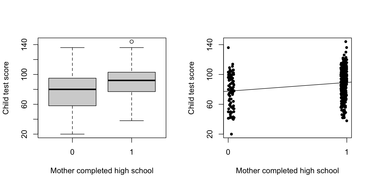
- We start by modeling the children’s test scores given an indicator for whether the mother graduated from high school (coded as 1) or no (coded as 0). The fitted is \[kid.score=78 + 12\cdot mom.hs + error,\] but for now we focus on the deterministic part, \[\hat{kid.score} = 78 + 12\cdot mom.hs,\] where \(\hat{kid.score}\) denotes either predicted or expected test score given the \(mom.hs\) predictor.
- 이 모형은 고등학교를 졸업한 어머니를 둔 아동과 그렇지 않은 어머니를 둔 아동 간의 평균 시험 점수 차이를 요약한 것이라 할 수 있음
- From the regression line:
- \(E[kid.score|mom.hs=0] = 78\)
- \(E[kid.score|mom.hs=1] = 78 + 12=90\)
- 고등학교를 졸업한 어머니의 자녀가 고등학교를 졸업하지 않은 어머니의 자녀보다 평균적으로 12점 더 높은 점수를 받는다는 것을 의미
5.1.2 A continuous predictor
fit.1 <- lm (kid_score ~ mom_iq)

plot(mom_iq,kid_score, xlab="Mother IQ score",
  ylab="Child test score",pch=20, xaxt="n", yaxt="n"
  , col=rgb(0, 0, 1, alpha = 0.3)
  , main='with regression line')
axis (1, c(80,100,120,140))
axis (2, c(20,60,100,140))
abline (fit.1)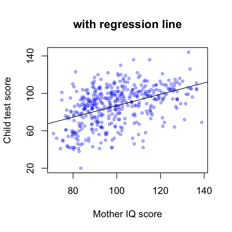
If we regress instead on continuous predictor, mother’s score on an IQ test, the fitted model is \[kid.score=26 + 0.6\cdot mom.iq + error.\]
이 점들은 주어진 어머니의 IQ 수준에서 예측된 아동의 시험 점수로 볼 수도 있고, 해당 IQ 점수로 정의된 하위집단의 평균 시험 점수로 해석할 수도 있음.
어머니의 IQ가 1점 차이 나는 하위집단 간의 아동 평균 점수를 비교하면, 어머니의 IQ가 더 높은 집단의 아동이 평균적으로 0.6점 더 높은 점수를 받을 것으로 기대.
더 흥미롭게 들리는 표현: 어머니의 IQ가 10점 차이 나는 두 아동 집단 간에는, 아동의 시험 점수도 평균적으로 6점 차이 날 것으로 예상.
절편 항(intercept)은 그리 유용한 값은 아닙니다: 어머니의 IQ가 0일 때 기대되는 아동의 시험 점수이기 때문 :(
5.2 Multiple predictors
fit.2 <- lm (kid_score ~ mom_hs + mom_iq)

plot(mom_iq,kid_score, xlab="Mother IQ score",
  ylab="Child test score",pch=20, xaxt="n", yaxt="n", type="n")
curve (coef(fit.2)[1] + coef(fit.2)[2] + coef(fit.2)[3]*x, add=TRUE, col=rgb(0, 1, 1))
curve (coef(fit.2)[1] + coef(fit.2)[3]*x, add=TRUE,col=rgb(0, 0, 1))
points (mom_iq[mom_hs==0], kid_score[mom_hs==0], pch=16, col=rgb(0, 0, 1, alpha = 0.3))
points (mom_iq[mom_hs==1], kid_score[mom_hs==1], col=rgb(0, 1, 1, alpha = 0.3), pch=16)
axis (1, c(80,100,120,140))
axis (2, c(20,60,100,140))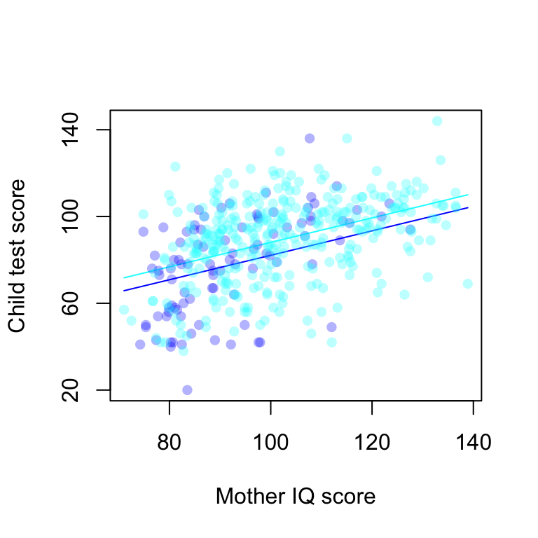
Consider a linear regression predicting child test scores from maternal education and maternal IQ. The fitted model is \[kd.score=26+6\cdot mom.hs + 0.6\cdot mom.iq+error.\]
- This model forces the slope of the regression of child’s test score on mother’s IQ score to be the same for each maternal education subgroup.
- We interpret the coefficients:
- Intercept: If a child had a mom with an IQ of 0 and who did not complete high school, then we would predict this child’s test score to be 26 :(
- Coefficient for \(mom.hs\): Comparing children whose moms have the sameIQ, but who differed in whether they completed high school, the model predicts an expected difference of 6 in their test scores.
- Coefficient for \(mom.iq\): Comparing children with moms have the same education level, but whose moms differ by 10 point in IQ, we would expect to see a difference of 6 points in the child’s test score.
이 모델은 어머니의 교육 수준 하위 그룹마다 아동의 시험 점수를 어머니 IQ에 대해 회귀시킬 때 기울기가 동일하도록 설정.
계수 해석:
절편: 어머니의 IQ가 0이고 고등학교를 졸업하지 않은 경우, 해당 아동의 시험 점수는 26점으로 예측됨. 😟
\(mom.hs\)의 계수: 어머니의 IQ가 동일하지만 고등학교 졸업 여부가 다른 두 아동을 비교할 때, 고등학교를 졸업한 어머니를 둔 아동의 시험 점수가 평균적으로 6점 더 높을 것으로 예측됨.
\(mom.iq\)의 계수: 어머니의 교육 수준이 동일하지만 IQ가 10점 차이 나는 경우, 아동의 시험 점수도 평균적으로 6점 차이 날 것으로 예측됨.
Caveat
모든 다른 변수를 고정한 채 하나의 예측 변수를 변화시키는 것이 항상 가능한 것은 아니다.
어떤 상황에서는 하나의 예측 변수의 값을 바꾸면서 다른 모든 변수를 고정하는 것이 논리적으로 불가능하다.
예: \(IQ\)와 \(IQ^2\)를 모두 예측 변수로 포함한 모델의 경우
반사실적(counterfactual) 해석과 예측(predictive) 해석
예측 해석은 관련된 예측 변수에서 1만큼 차이가 나는 두 집단(다른 모든 변수는 동일한)을 비교할 때, 결과 변수가 평균적으로 어떻게 달라지는지를 고려한다. 선형 모델 하에서는 회귀 계수가 이러한 두 집단 간 결과의 기대 차이를 나타낸다.
반사실적 해석은 개인 간 비교가 아닌, 개인 내의 변화를 전제로 한다. 이 해석에서 회귀 계수는 다른 모든 변수를 동일하게 유지한 채 해당 예측 변수를 1만큼 증가시켰을 때 결과 변수에 발생하는 기대 변화량이다. 예: “어머니의 IQ가 100에서 101로 증가하면 자녀의 점수가 평균적으로 0.6점 증가할 것이다.” 이러한 해석은 인과 추론에서 사용된다.
반사실적 해석을 하기 위해서는 Unconfoundedness, Positivity, Structural Stability과 같은 강한 가정이 필요하다.
이러한 가정이 충족되지 않는 경우, 우리는 단순한 연관(association)으로 해석해야 한다.
- 예: 어머니의 IQ가 10 증가하면 자녀의 점수가 6점 증가하는 것과 연관이 있다.
5.3 Interaction
What do you think about your model in Section 5.2. Do you think the assumption of eqaul slope is appropriate in your data? I think the slope for the purple line should be higher. Let’s remove the assumption.
## lm(formula = kid_score ~ mom_hs + mom_iq + mom_hs:mom_iq)
##               coef.est coef.se
## (Intercept)   -11.48    13.76
## mom_hs         51.27    15.34
## mom_iq          0.97     0.15
## mom_hs:mom_iq  -0.48     0.16
## ---
## n = 434, k = 4
## residual sd = 17.97, R-Squared = 0.23par(mfrow=c(1,2))
plot(mom_iq,kid_score, xlab="Mother IQ score",
ylab="Child test score",pch=20, xaxt="n", yaxt="n", type="n")
curve (coef(fit)[1] + coef(fit)[2] + (coef(fit)[3] + coef(fit)[4])*x, add=TRUE, col=rgb(0, 1, 1, alpha = 1))
curve (coef(fit)[1] + coef(fit)[3]*x, add=TRUE,col=rgb(0, 0, 1, alpha = 1))
points (mom_iq[mom_hs==0], kid_score[mom_hs==0], pch=20,col=rgb(0, 0, 1, alpha = 0.3))
points (mom_iq[mom_hs==1], kid_score[mom_hs==1], col=rgb(0, 1, 1, alpha = 0.3), pch=20)
axis (1, c(80,100,120,140))
axis (2, c(20,60,100,140))
plot(mom_iq,kid_score, xlab="Mother IQ score",
ylab="Child test score",pch=20, type="n", xlim=c(0,150), ylim=c(0,150), main='x-axis extended to zero to show intercept',cex.main=0.8)
curve (coef(fit)[1] + coef(fit)[2] + (coef(fit)[3] + coef(fit)[4])*x, add=TRUE, col=rgb(0, 1, 1, alpha = 1))
curve (coef(fit)[1] + coef(fit)[3]*x, add=TRUE,col=rgb(0, 0, 1, alpha = 1))
points (mom_iq[mom_hs==0], kid_score[mom_hs==0], pch=20,col=rgb(0, 0, 1, alpha = 0.3))
points (mom_iq[mom_hs==1], kid_score[mom_hs==1], col=rgb(0, 1, 1, alpha = 0.3), pch=20)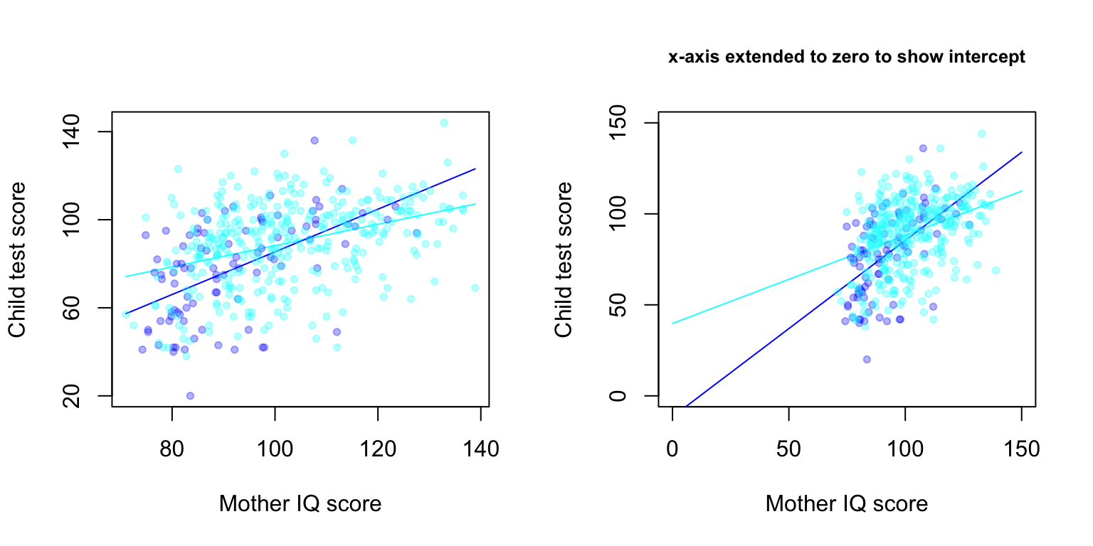
A remedy is to include interaction! The fitted model is: \[kid.score = -11 + 51\cdot mom.hs + 1.1 \cdot mom.iq - 0.5\cdot mom.hs\cdot mom.iq + error.\]
- Some coefficients are not easily interpretable.
- We can understand the model as two separate regression lines as the figure.
- For children whose mom did not finish high school: \[\hat{kid.score} = -11 + 1.1\cdot mom.iq \]
- For children whose mom finish high school” \[\hat{kid.score}=(-11+51) + (1.1-0.5)\cdot mom.iq\]
Note
- When should we look for interactions?
- predictors that have large main effects also tend to have large interactions with other predictors (However, small main effects does not preclude large interactions)
5.4 Statistical Inference
5.4.1 Writing Model
When illustrating specific examples, it helps to use descriptive variable names.
But now its time to discuss general theory. We adopt generic mathematical notations.
We define \(n\times p\) design matrix \(X\) with the row vectors \(X_1,\ldots X_n\in R^p\) (without the column corresponding to the intercept term).
Each row vector \(X_i\) includes elements \(X_{ij}\) for \(j=1,\ldots,p\).
\(y\in R^n\) is the observed outcome vector.
\(I\) is the identity matrix with fixed dimension.
Three ways of writing the model:
- \[y_i = X_i\beta + \epsilon_i = \beta_0 + \beta_1X_{i1}+\ldots+\beta_pX_{ip}+\epsilon_i, \textrm{ for } i=1,\ldots,n ,\] where errors \(\epsilon_i\) have independent normal distributions with mean 0 and standard deviation \(\sigma\).
- \[y_i \sim N(X_i\beta,\sigma^2), \textrm{ for } i=1,\ldots,n.\]
- \[y\sim N(X\beta,\sigma^2I)\]
5.4.2 Fitting
Read the data:
kidiq <- read.dta("GelmanData/kidiq.dta") # Read stata file
attach(kidiq)
The lm function fits linear models.
##
## Call:
## lm(formula = kid_score ~ mom_hs + mom_iq + mom_hs:mom_iq)
##
## Residuals:
##     Min      1Q  Median      3Q     Max
## -52.092 -11.332   2.066  11.663  43.880
##
## Coefficients:
##               Estimate Std. Error t value Pr(>|t|)
## (Intercept)   -11.4820    13.7580  -0.835 0.404422
## mom_hs         51.2682    15.3376   3.343 0.000902 ***
## mom_iq          0.9689     0.1483   6.531 1.84e-10 ***
## mom_hs:mom_iq  -0.4843     0.1622  -2.985 0.002994 **
## ---
## Signif. codes:  0 '***' 0.001 '**' 0.01 '*' 0.05 '.' 0.1 ' ' 1
##
## Residual standard error: 17.97 on 430 degrees of freedom
## Multiple R-squared:  0.2301, Adjusted R-squared:  0.2247
## F-statistic: 42.84 on 3 and 430 DF,  p-value: < 2.2e-16
5.4.2.1 Least squares estimation of \(\beta\)
For the model \(y = X\beta+\epsilon\), the least squares estimate is the \(\hat{\beta}\) that minimizes the sum of squared errors, \(\sum_{i=1}^n(y_i-X_i\hat{\beta})^2\). We have a closed form solution: \((X^TX)^{-1}X^Ty\).
You can implement it without using the lm() function.
X <- model.matrix(~mom_hs + mom_iq + mom_hs:mom_iq)
y <- kid_score
hbeta <- solve(t(X)%*%X)%*%t(X)%*%y
Compare this one with the result from lm() function.
DIY Go back to the iris assignment. If you used lm() function in the permutation procedure. Correct. It will be much more efficient. There are even more efficient ways using low-rank decomposition. Describe and implement it.
5.4.2.2 Uncertainty
How do you derive standard error of \(\beta\) theoretically? We start from the OLS form.
- \(\hat{\beta} = (X^TX)^{-1}X^Ty\)
- Plug-in the model on \(y\): \(\hat{\beta}=(X^TX)^{-1}X^T(X\beta+\epsilon)\)
- The random variable \(\epsilon\) induces distribution of \(\hat{\beta}\) \[\hat{\beta}\sim N(\beta,\sigma^2(X^TX)^{-1})\]
- \(Var(\hat{\beta}) = \sigma^2(X^TX)^{-1}\)
So we should know \(\sigma^2\) to make inference on \(\beta\).
- Consider residuals \(r_i= y_i - X_i\hat{\beta}\), that they are assumed to be normal.
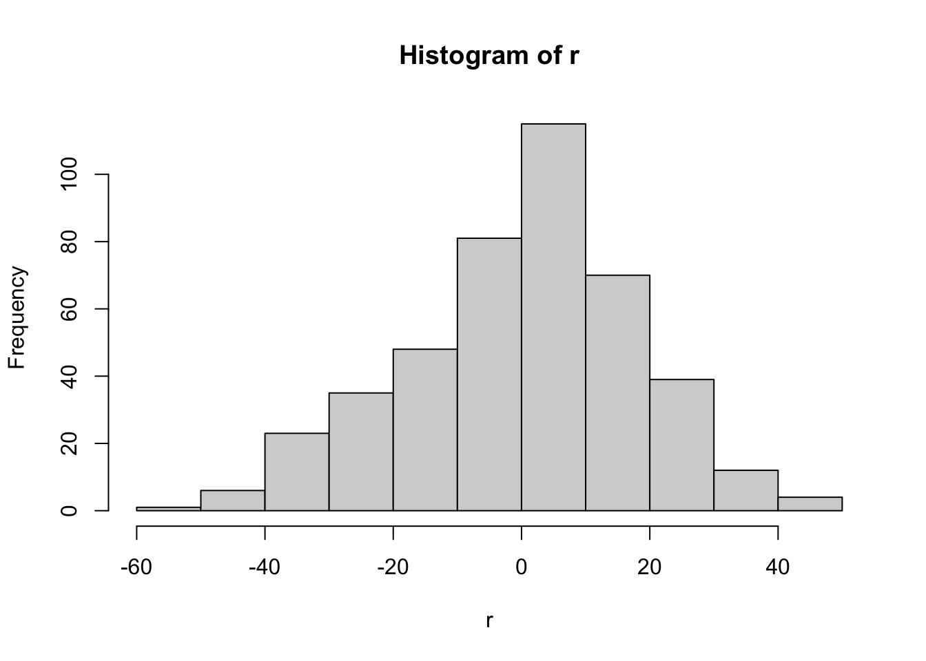
- Calculate residual standard deviation, \(\hat{\sigma} = \sqrt{\sum_{i=1}^n r_i^2/(n-p)}\)
- Compute standard errors for regression coefficients:
##   (Intercept)        mom_hs        mom_iq mom_hs:mom_iq
##    13.7579737    15.3375805     0.1483437     0.1622171
We can construct a rough confidence interval \(\hat{\beta}_j \pm 2 \cdot se(\hat{\beta}_j)\).
- As you see they are correlated. Calculate correlation:
We’re not using covariance for inference, but it is often used for simulations (we will see later).
DIY Check the ‘arm::sim’ function.
5.4.2.3 Goodness of fit
The fit of the model can be summarized by
- \(\hat{\sigma}^2\) (the smaller the better fit). But there’s no upper bound.
- \(R^2\), the fraction of variance explained by the model: \[R^2 = 1-\hat{\sigma}^2/s_y^2 \textrm{ or } R^2_{adj}=1-\frac{(1-R^2)(n-1)}{n-p-2}\] where \(s_y^2\) as the SD of \(y\).
Is the result disapointing that the model explains about 22% of the total variance? However it is a good thing: a child’s achievement cannot be accurately predicted given only these maternal characteristics.
5.4.2.4 Use ggplot2 for better display
library(tidyverse)
ggplot(kidiq, aes(x = mom_iq, y = kid_score)) +
  geom_point(alpha = 0.6) +
  geom_smooth(method = "lm", se = TRUE, color = "blue", fill = "lightblue",level=0.99) +
  labs(title = "Regression Line with Confidence Interval",
       x = "Mom IQ",
       y = "Kid IQ") +
  theme_minimal()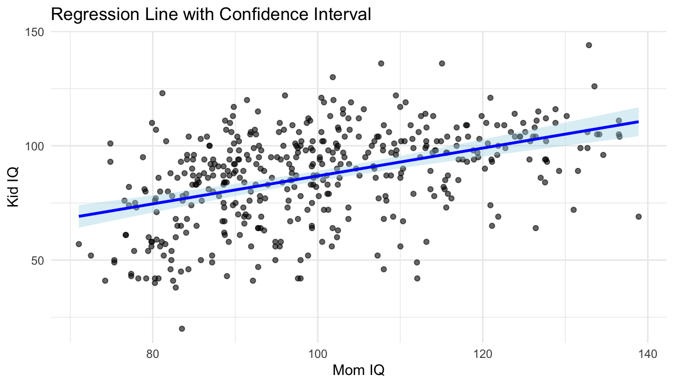
You can observe that the width of the confidence band varies across values of x; it tends to be wider in regions with fewer data points. This is because the confidence interval is constructed based on the standard error of the predicted mean, which increases as the distance from the mean of x increases or as data becomes sparse in those regions.
DIY Show how to construct the confidence band.
5.5 Assumptions and Diagnostics
Some assumptions may not be testable from the available data alone!
- Additivity and linearity
- Independence of errors
- equal variance of errors
- Normality of errors
Plotting residuals to reveal aspects of the data not captured by the model:
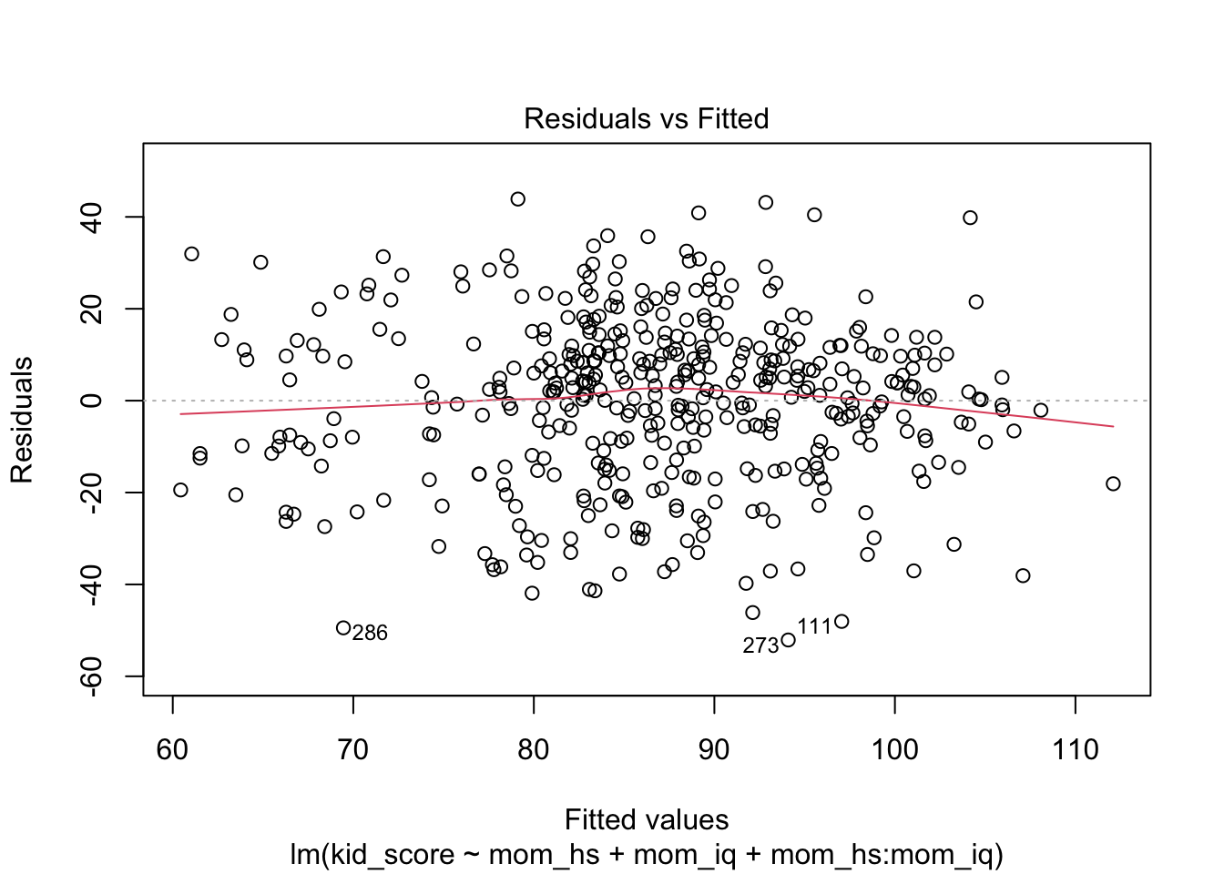
- Residual vs. Fitted
- Purpose: linearity and homoscedasticity
- Interpretation:
- The points should be randomly scattered around the horizontal line (residual =0)
- If you see a curve, the model may be missing a nonlinear term
- If the spread grows or shrinks: sign of Heteroscedasticity
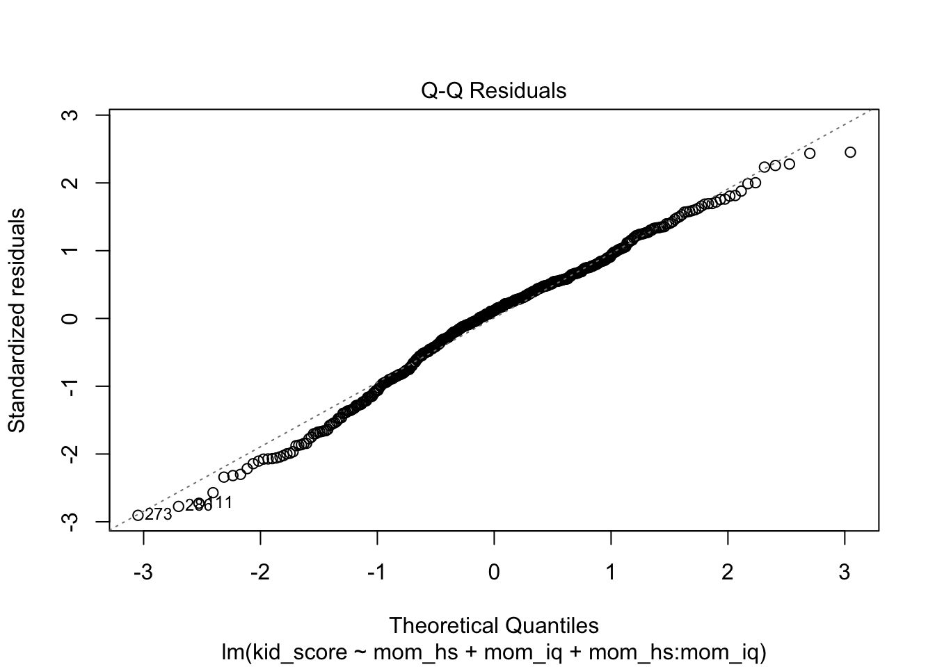
- Q-Q plot
- Purpose: Normality
- Interpretation: Minor deviations are ok
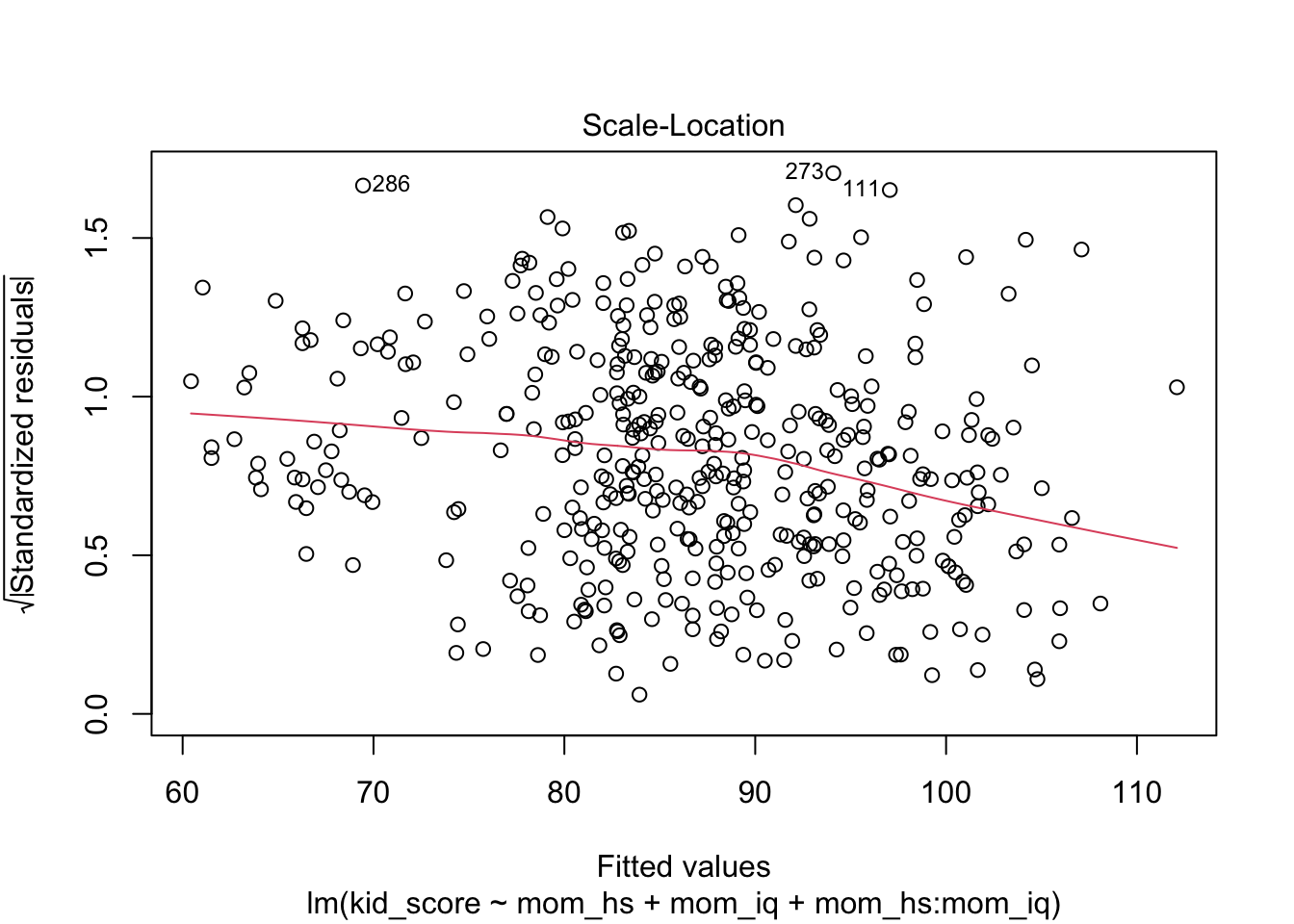
- Scale-Location Plot
- Purpose: Homoscedasticity
- Interpretation: If you see a funnel shape, variance is not constant
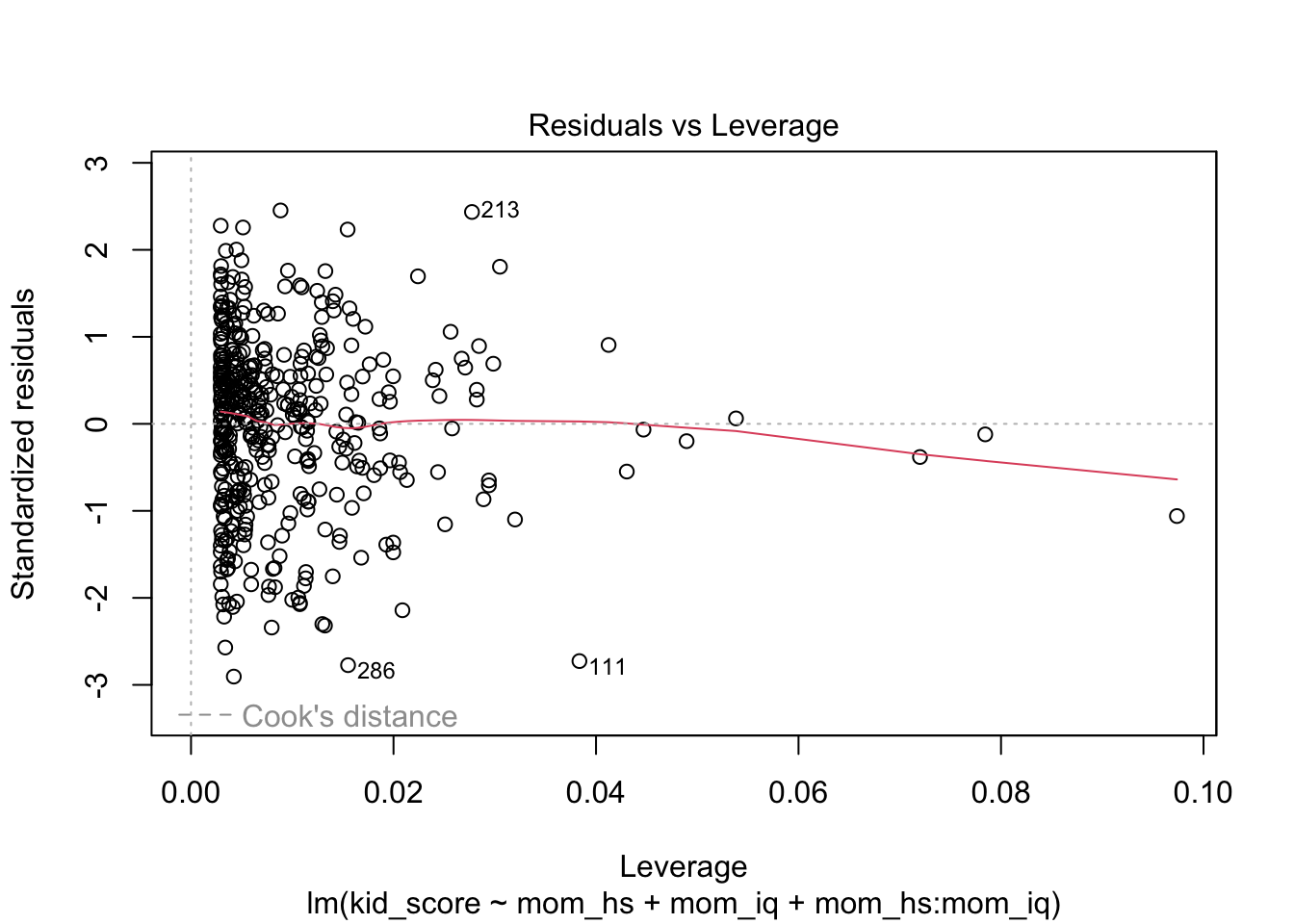
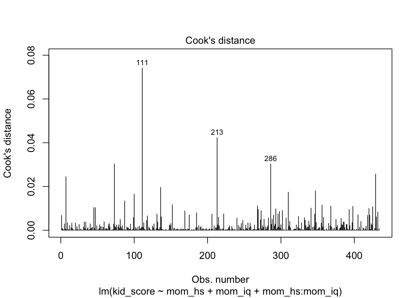
- Residuals vs Leverage
- Purpose: Identifies influential points
- Interpretation: Points with high leverage and large residuals are influential
Note The leverage for a sample \(i\), \(h_i\) is the corresponding diagonal element of the hat matrix \(H = X(X^TX)^{-1}X^T\). The Cook’s distance for each individual \(i\) is \(D_i = \frac{r_i^2}{p\cdot \hat{\sigma}^2} \cdot \frac{h_i}{(1-h_i)^2}\).
5.6 DIY: Simulation
Evaluate the Type I error rate and power of the simple linear regression procedure. Investigate how the performance changes when the normality assumption is violated.
Apply a permutation test to the same setting, and evaluate its Type I error rate and power. Compare the performance of the permutation test to that of the simple linear regression procedure discussed above.