Chapter 9 The Bootstrap

This lecture is based on:

• L. Wasserman. All of Statistics. Springer, 2010.
• G. James, D. Witten, T. Hastie, R. Tibshirani. An Introduction to Statistical Learning with Applications in R. Chapter 5. Springer, 2013.
• B. Efron and R.J. Tibshirani. An introduction to the Bootstrap. Chapman & Hall, 2010.
• A.W. van der Vaart. Asymptotic Statistics. Chapter 23. Cambridge University Press, 1998.
• A. DasGupta. Asymptotic Theory of Statistics and Probability. Chapter 29. Springer, 2008.

The Bootstrap belongs to the wider class of resampling methods.

• It was introduced in 1979 by Bradley Efron and offered a principled, simulation-based approach for measures of accuracy to statistical estimates, and estimating biases, variances or obtaining appropriate confidence intervals.

• It applies to both parametric (when the distribution of the data is known and parameterized by a finite-dimensional parameter) and nonparametric settings.

9.1 Motivating Examples

9.1.1 Confidence interval for the median of a population

Let \(X_1,X_2,\ldots, X_n\) be independent identically distributed (iid) random variables from a cumulative distribution function (cdf) \(F\) and consider that we are interested in the median \(m=F^{-1}(0.5)\) of the distribution. We consider the following estimator \[ \hat{M}_n = \begin{cases} X_{(n+1)/2} & \text{if } n \text{ odd},\\ \frac{1}{2}(X_{n/2} + X_{n/2+1}) & \text{if } n \text{ even}, \end{cases} \] where \(X_{r}\) is the \(r\)th order statistic of the random sample \((X_1,\ldots,X_n).\)

Example 1(Wages). We are interested in the median wage in the mid-Atlantic states of the USA in 2005. We consider the dataset from the R packages ISLR, which consists of the wages of \(n=447\) workers in that region in 2005.

library(ISLR)
data(Wage)
wage2005 = Wage$wage[Wage$year==2005]
length(wage2005)

## [1] 447

hist(wage2005)

mhat = median(wage2005)
mhat

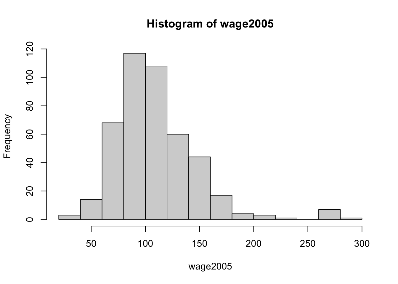
## [1] 104.9215

The median estimate is just a point estimate for the population median \(m\). How do we get a confidence interval for \(m\)? If \(F\) is differentiable with probability density function (pdf) \(f\), then the asymptotic distribution \(\hat{M}_n\) is \[\sqrt{n}(\hat{M}_n - m ) \rightarrow_d \textit{N}(0, \frac{1}{4f^2(m)}),\] as \(n\rightarrow \infty\).

• We cannot evaluate the variance term due to the unknown density \(f\)
• If we could evaluate \(\sigma^2 = \mathbb{V}(\hat{M}_n)\), then we could use the normal approximation to obtain an approximate \(1-\alpha\) confidence interval. The bootstrap allows to obtain an estimate of the variance \(\sigma^2\) of the estimator.
• Alternatively, if we knew the quantiles \(q_{\alpha/2}\) and \(q_{1-\alpha/2}\) of the distribution of \(\hat{M}_n - m\) where \[P(\hat{M}_n-m \leq q_x) = x\] for \(x\in [0,1]\), then we could use these quantiles to build a \(1-\alpha\) confidence interval \([\hat{M}_n-q_{1-\alpha/2},\hat{M}_n-q_{\alpha/2}]\) for \(m\) as \[P(q_{\alpha/2}\leq \hat{M}_n - m \leq q_{1-\alpha/2}) = 1-\alpha.\] The quantiles are also in general impossible to obtain analytically. The bootstrap provides estimates of the quantiles \(q_{\alpha/2}\) and \(q_{1-\alpha/2}\) and thus approximate confidence intervals.

9.1.2 Bias and Variance of an estimator

Let \(X_1,\ldots,X_n\) be iid random variables from a pdf \(f(x;\theta)\) parametrized by \(\theta\). Let \[\hat{\theta}_n = t(X_1,\ldots,X_n)\] be some estimator of \(\theta\).

• In order to evaluate the accuracy of the estimator, we may be interested in evaluating

  • Bias: \(E[\hat{\theta}_n]-\theta\)
  • Variance: \(Var(\hat{\theta}_n).\)

• The bootstrap is a general strategy to obtain estimates for these quantities. And the CIs.

9.2 Background

9.2.1 Satistical functional

A statistical functional \(\mathcal{F}(F)\) is any function of the cdf \(F\). Examples include

• the mean \(E(X) = \int x dF(x)\)
• the variance \(Var(X) = \int x^2 dF(x) - (\int x dF(x))^2\)
• the median \(m=F^{-1}(0.5)\).

9.2.2 Empirical distribution function

Let \(X_1,\ldots, X_n\) be iid real-valued random variables with cdf \(F\). The empirical cumulative distribution function is defined as \[F_n(x) = \frac{1}{n}\sum_{i=1}^nI(X_i\leq x) = \frac{\#|\{i|X_i\leq x\}|}{n}.\]

The empirical cdf have the following attractive theoretical properties: \(F_n(x)\) is

1. Unbiasedness
   \[ E\bigl[F_n(x)\bigr] = F(x),\quad \forall x\in\mathbb{R}. \]

2. Strong consistency
   \[ F_n(x)\xrightarrow{\mathrm{a.s.}}F(x),\quad n\to\infty. \]

3. Asymptotic normality
   \[ \sqrt{n}\bigl(F_n(x)-F(x)\bigr) \xrightarrow{d} N\bigl(0,\;F(x)\{1-F(x)\}\bigr). \]

proof. For any \(x\in \mathbb{R}\), the binary random variables \(I(X_i\leq x) \text{ } \forall i\) are independent and identically Bernoulli distributed with success probability of \(F(x)\). Hence the discrete random variable \(nF_n(x) \sim Binomial(n,F(x))\) and (i) follows. (ii) follows from the strong large numbers and (iii) by CLT.

ecdf.wages = ecdf(wage2005)
plot(ecdf.wages, xlab = 'x', ylab = 'Fn(x)', main = 'Empirical cdf', col='lightblue2')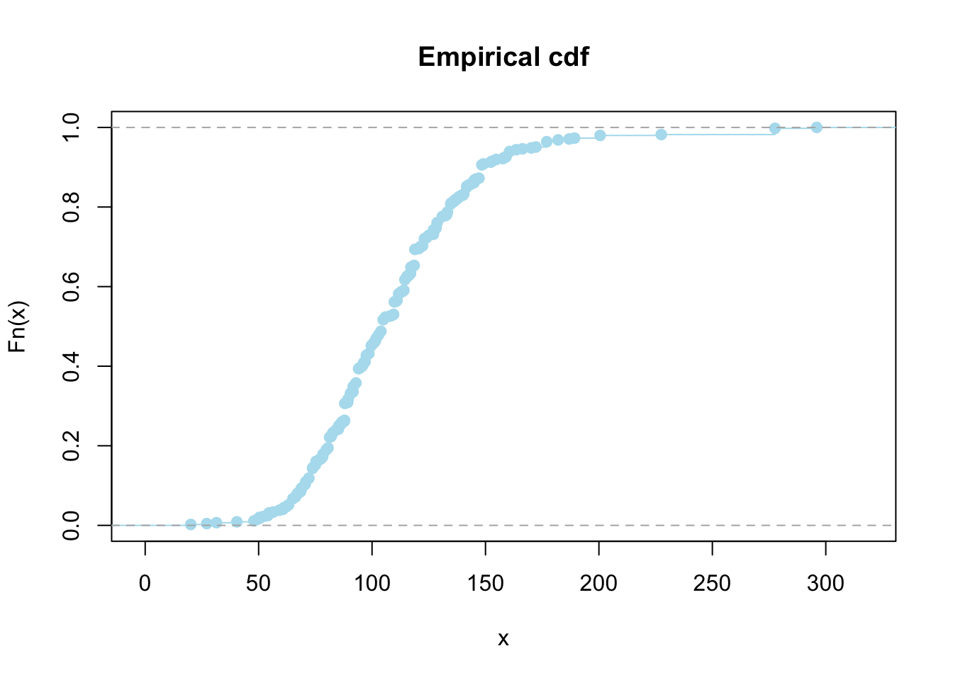

9.2.3 Monte Carlo Integration

The Monte Carlo method is a way to approximtate potentially high-dimensional integrals via simulation.

Let \(Y \in \mathbb{R}^p\) be a continuous or discrete random variable with cdf \(G\). Consider \[\eta = E(\phi(Y)) = \int_{\mathbb{R}^p} \phi(y)dG(y)\] where \(\phi:\mathbb{R}^p \rightarrow \mathbb{R}\). Let \(Y^{(1)},\ldots, Y^{(B)}\) be iid random variables with cdf \(G\). Then \[\hat{\eta}_B = \frac{1}{B} \sum_{j=1}^B \phi(Y^{(j)})\] is called the Monte Carlo estimator of the expectation \(\eta\).

The Monte Carlo algorithm, which only requires to be able to simulate from \(G\), is as follows:

---

Algorithm 1: Monte Carlo Algorithm

1. Simulate independent \(Y^{(1)},\ldots Y^{(B)}\) with cdf \(G\)

2. Return \(\hat{\eta}_B = \frac{1}{B}\sum_{j=1}^B \phi(Y^{(j)})\).

---

Here are the properties of the Monte Carlo estimator, which follow from the law of large numbers and the central limit theorem.

Proposition 5. The Monte Carlo estimator is

1. (i) Unbiased
   \[ \mathbb{E}(\hat{\eta}_B) = \eta \quad \text{for any } B \geq 1. \]

2. (ii) (Strongly) consistent
   \[ \hat{\eta}_B \xrightarrow{a.s.} \eta \quad \text{as } B \to \infty, \]

3. (iii) Asymptotically normal.
   If \(\sigma^2 = \mathbb{V}(\phi(Y))\) exists, then \[ \sqrt{B}(\hat{\eta}_B - \eta) \xrightarrow{d} \mathcal{N}(0, \sigma^2) \quad \text{as } B \to \infty. \]

For example, the Monte Carlo estimators of the mean and variance of \(Y\) are:

\[ \hat{\mu}_B = \frac{1}{B} \sum_{j=1}^B Y^{(j)} \xrightarrow{a.s.} \mathbb{E}(Y), \]

\[ \hat{\sigma}^2_B = \frac{1}{B} \sum_{j=1}^B \left(Y^{(j)} - \hat{\mu}_B \right)^2 \]

\[ = \frac{1}{B} \sum_{j=1}^B (Y^{(j)})^2 - \left( \frac{1}{B} \sum_{j=1}^B Y^{(j)} \right)^2 \xrightarrow{a.s.} \mathbb{V}(Y). \]

9.3 Bootstrap

Let \(X_1,\ldots, X_n\) be iid random variables with cdf \(F\). The distribution \(F\) of the data is unknown, and we cannot even simulate from \(F\). Consider the estimator \[\hat{\theta}_n = t(X_1,\ldots,X_n)\] for estimating \(\theta =\mathcal{F}(F)\) a statistical functional of \(F\). This setup is represented below: \[\text{Real World: } F \Rightarrow X_1,\ldots,X_n \Rightarrow \hat{\theta}_n = t(X_1,\ldots,X_n)\]

9.3.1 Variance Estimation

We are first interested in estimating the variance \(\sigma^2 = \mathbb{V}_F(\hat{\theta}_n)\) of the estimator \(\hat{\theta}_n\). We write \(\mathbb{V}_F\) to emphasize the fact that the variance depends on the unknown cdf \(F\).

9.3.1.1 An idealized variance estimator

Suppose first that we could simulate from the cdf \(F\), that is we could reproduce the Real World and generate new datasets. Then we could use the Monte Carlo method to obtain a Monte Carlo estimator for \(\sigma^2\) as follows.

• For \(j = 1, \dots, B\):
  • Let \(X_1^{(j)}, \dots, X_n^{(j)}\) be iid from \(F\) and \(\hat{\theta}_n^{(j)} = t(X_1^{(j)}, \dots, X_n^{(j)})\)
• The Monte Carlo variance estimator is \[ \hat{\sigma}^2_{n,B} = \frac{1}{B} \sum_{j=1}^B \left( \hat{\theta}_n^{(j)} - \frac{1}{B} \sum_{j=1}^B \hat{\theta}_n^{(j)} \right)^2. \]

However, the cdf \(F\) is unknown and we cannot simulate from it, so we cannot implement this estimator.

9.3.1.2 The bootstrap for variance estimation

The idea of the bootstrap is to:

1. Replace the unknown cdf \(F\) by its (known) empirical cdf \(F_n\)
2. Use the Monte Carlo method.

More formally, conditionally on \(X_1, \dots, X_n\), let \(X_1^*, \dots, X_n^*\) be iid random variables with cdf \(F_n\) and \[ \hat{\theta}_n^* = t(X_1^*, \dots, X_n^*). \] The bootstrap mimics the Real World by using the empirical cdf \(F_n\):

• Real World: \(F \Rightarrow X_1, \dots, X_n \Rightarrow \hat{\theta}_n = t(X_1, \dots, X_n)\)
  
• Bootstrap World: \(F_n \Rightarrow X_1^*, \dots, X_n^* \Rightarrow \hat{\theta}_n^* = t(X_1^*, \dots, X_n^*)\)

The bootstrap relies on two approximations:

1. Approximate \(\mathbb{V}_F(\hat{\theta}_n)\) by \(\mathbb{V}_{F_n}(\hat{\theta}_n^*)\) using \(F_n\)
2. Approximate \(\mathbb{V}_{F_n}(\hat{\theta}_n^*)\) by Monte Carlo to obtain the bootstrap estimate \(\hat{\sigma}^2_{n,B}\)

In a nutshell:

\[ \mathbb{V}_F(\hat{\theta}_n) \overset{\text{Empirical cdf}}{\simeq} \mathbb{V}_{F_n}(\hat{\theta}_n^*) \overset{\text{Monte Carlo}}{\simeq} \hat{\sigma}^2_{n,B} \]

• Simulating \(X_1^*, \dots, X_n^*\) from \(F_n\) is easy. \(F_n\) puts mass \(1/n\) at each value \(\{X_1, \dots, X_n\}\).

• \(X_1^*, \dots, X_n^*\) are thus discrete random variables, and we can simulate from \(F_n\) by sampling with replacement from the original dataset \(\{X_1, \dots, X_n\}\).

---

Algorithm 2: Bootstrap algorithm for estimating the variance

Let \(X_1, \dots, X_n\) be some data and \(\hat{\theta}_n = t(X_1, \dots, X_n)\).

• For \(j = 1, \dots, B\):
  • Simulate \(X_1^{*(j)}, \dots, X_n^{*(j)} \sim_{iid} F_n\) by sampling with replacement from \(\{X_1, \dots, X_n\}\)
  • Evaluate \(\hat{\theta}_n^{*(j)} = t(X_1^{*(j)}, \dots, X_n^{*(j)})\)
• Return the bootstrap variance estimate \[ \hat{\sigma}^2_{n,B} = \frac{1}{B} \sum_{j=1}^B \left( \hat{\theta}_n^{*(j)} - \frac{1}{B} \sum_{j=1}^B \hat{\theta}_n^{*(j)} \right)^2 \]

---

9.3.1.3 Example

Consider the median estiamator \(\hat{M}_n\) to estimate its variance \(\mathbb{V}_F(\hat{M}_n)\).

bootstrap_variance_median <- function(X, B) {
  # Bootstrap variance estimate for the median estimator
  # X: Data
  # B: Number of Monte Carlo samples
  n <- length(X)
  mhat.boot <- numeric(B) 

  for (j in 1:B){
    X.boot <- sample(X,n,replace=TRUE) # Sample bootstrap data from Fn
    mhat.boot[j] <- median(X.boot) # Median bootstrap samples 
  }
  var.boot <- var(mhat.boot) # Evaluate the bootstrap variance estimate
  return(list(var.boot = var.boot, mhat.boot = mhat.boot)) 
}

We start with a synthetic normal dataset with \(n=500\). * \(X_1,\ldots,X_n\) are normally distributed with mean 0.4 and variance 1.

n <- 500
X <- rnorm(n,mean=0.4) # Median estimate mhat.gauss <- median(X)
# Median estimate 
mhat.gauss <- median(X)

We now estimate the variance of the median estimator using the bootstrap.

B <- 10000
results.gauss = bootstrap_variance_median(X,B)
mhat.boot.gauss = results.gauss$mhat.boot
hist(mhat.boot.gauss, xlab='mhat.boot', main='',col='orange', breaks=20)
points(mhat.gauss,0,pch = 22,col='red',bg='red')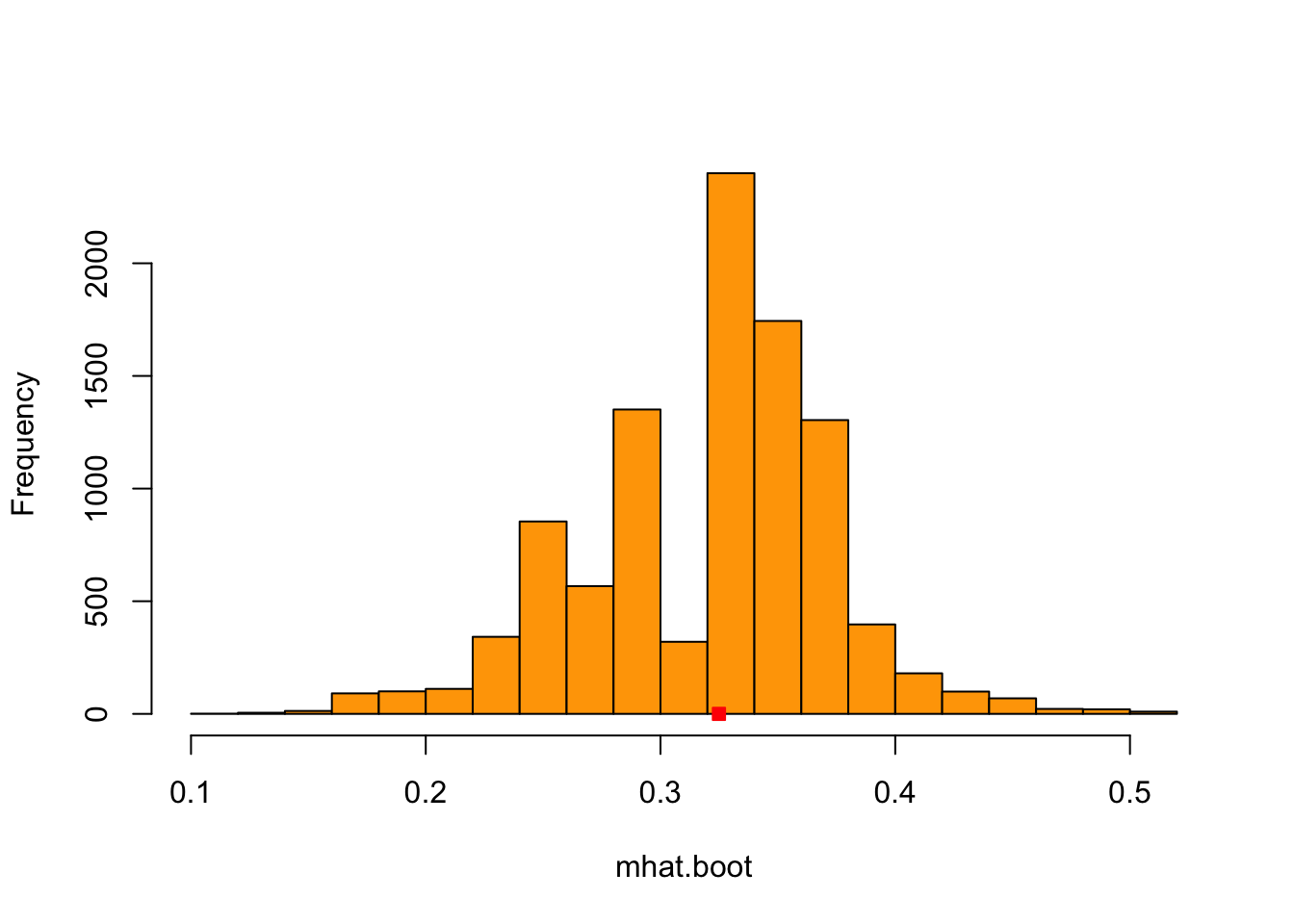

This is the histogram of the \(B=10000\) bootstrap samples \(\hat{M}_n^{*(1)},\ldots, \hat{M}_n^{*(B)}\) of the median estimator and the red square is \(\hat{M}_n\) for the Gaussian synthetic dataset.

var.boot.gauss = results.gauss$var.boot
var.boot.gauss

## [1] 0.002706442

DIY Compare it with the theoretical one. Because this is from synthetic data, we know the true distribution \(F\). So we can evaluate how accurate the bootstrap variance is.

We now consider the wages dataset and use the bootstrap estimator to estimate the variance of the sample median.

B <- 10000
results.wages <- bootstrap_variance_median(wage2005,B)
mhat.boot.wages <- results.wages$mhat.boot
hist(mhat.boot.wages,xlab='mhat.boot', main='',col='orange', breaks=20)
points(mhat,0,pch = 22,col='red',bg='red')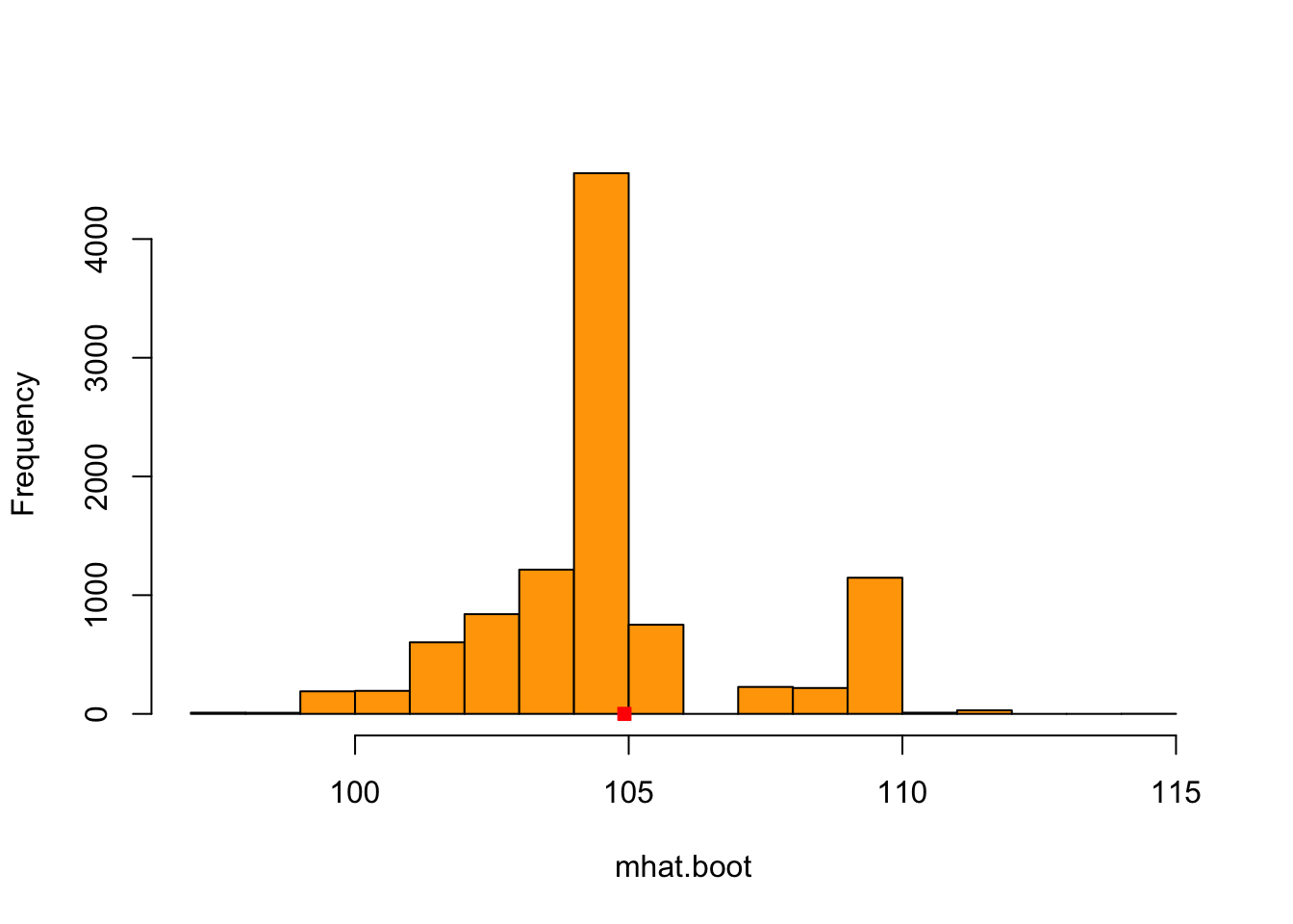

This is the histogram of the \(B=10000\) bootstrap samples \(\hat{M}_n^{*(1)},\ldots, \hat{M}_n^{*(B)}\) of the median estimator and the red square is \(\hat{M}_n\) for the wages dataset.

var.boot.wages = results.wages$var.boot
var.boot.wages

## [1] 5.543813

9.3.1.4 Confidence Intervals

Normal Approximation

If central limit theorem holds (iid, large \(n\)) for the estimator \(\hat{\theta}_n\), the following is statisfied: \[\frac{\hat{\theta}_n - \theta}{\sqrt{\mathbb{V}_F(\hat{\theta}_n)}} \rightarrow_d \mathcal{N}(0,1).\]

We can now approximate \(\mathbb{V}_F(\hat{\theta}_n)\) with \(\hat{\sigma}^2_{n,B}\). The \((1-alpha)\times 100\%\) bootstrap confidence interval is from :

\[P\left(z_{\alpha/2}<\frac{\hat{\theta}_n - \theta}{\hat{\sigma}^2_{n,B}}<z_{1-\alpha/2}\right) = 1-\alpha.\]

Thus, the confidence interval can be expressed as: \[\left(\hat{\theta}_n - z_{1-\alpha/2}\hat{\sigma}^2_{n,B},\hat{\theta}_n + z_{1-\alpha/2}\hat{\sigma}^2_{n,B}\right).\]

Now, we can construct the 95% confidence interval for the wages dataset.

alpha = 0.05
cm = qnorm(1-alpha/2) # Confidence multiplier
se = sqrt(var.boot.wages) # standard error of the statistics
me = cm * se # margin of error 
ci.bootnormal.wages = c(mhat - me,mhat + me)
ci.bootnormal.wages

## [1] 100.3067 109.5363

Bootstrap Pivotal Confidence Interval

• A pivotal quantity is a statistic whose distribution does not depende (or depends minimally) on unknown parameters.
• Consider the random variable (pivot) \(R_n = \hat{\theta}_n - \theta\).
• Let \(H_n(r) = P(R_n \leq r)\) be the (unknown) cdf of \(R_n\).
• \(H_n^{-1}\) is the associated quantile function \[q_\alpha := H_n^{-1}(\alpha) = inf\{x: H(x) >\alpha \}.\]
• To construct \(1-\alpha\) confidence interval, we can consider: \[1-\alpha = P(q_{\alpha/2}\leq \hat{\theta}_n-\theta\leq q_{1-\alpha/2})=P(\hat{\theta}_n - q_{1-\alpha/2}\leq \theta\leq \hat{\theta}_n - q_{\alpha/2}).\]
• However we do not know the quantiles.
• Here, we can use bootstrap to obtain an approximation of these quantiles.
• Bootstrap Approximation: \(R_n = \hat{\theta}_n - \theta\simeq R_n^* = \hat{\theta}^{*}_n - \hat{\theta}_n\).
• Consider the distribution: \(H_n^*(r) = P_{F_n}(R_n^*\leq r)\)
• This can be approximated by Monte Carlo methods to obtain the bootstrap estimate \[\hat{H}^{*}_{n,B}(r) =\frac{1}{B} \sum_{j=1}^B I(R_n^{*(j)}\leq r),\] where \(R_n^{*(j)} = \hat{\theta}^{*(j)}_n - \hat{\theta}_n.\)
• In a nutshell:

\[ H_n \overset{\text{Empirical cdf}}{\simeq} H_n^* \overset{\text{Monte Carlo}}{\simeq} \hat{H}^*_{n,B} \]

• We can obtain the quantiles based on these approximations: \[\hat{q}^*_\alpha =\hat{H}^{*-1}_{n,B}(\alpha)\] and build the bootstrap pivotal \(1-\alpha\) confidence interval \[C_n^* = [\hat{\theta}_n -\hat{q}^*_{1-\alpha/2},\hat{\theta}_n -\hat{q}^*_{\alpha/2}].\]

• As \(R_n^{*(j)} = \hat{\theta}_n^{*(j)} - \hat{\theta}_n\), we have \(\hat{q}^{*}_\alpha=\hat{q}^{\theta*}_\alpha - \hat{\theta}_n\), where \(\hat{q}^{\theta*}_\alpha\) is the \(\alpha\) quantile of the bootstrap samples \((\hat{\theta}^{*(1)},\ldots \hat{\theta}^{*(B)})\).

• Thus, in terms of \((\hat{\theta}^{*(1)},\ldots \hat{\theta}^{*(B)})\), the \(1-\alpha\) bootstrap pivotal confidence interval is given by \[C_n^* = [2\hat{\theta}_n-\hat{q}^{\theta*}_{1-\alpha/2}, 2\hat{\theta}_n-\hat{q}^{\theta*}_{\alpha/2}].\]

• Construct the 95% bootstrap pivotal CI.

ci.bootpivot.wages = c(2*mhat-quantile(mhat.boot.wages, 1-alpha/2,names=FALSE) ,
                 2*mhat-quantile(mhat.boot.wages,alpha/2,names=FALSE))
print(ci.bootpivot.wages)

## [1] 100.0090 109.0787

9.3.2 Bias Estimation

The bias of an estimator \(\hat{\theta}_n\) is \[b:=E_F(\hat{\theta}_n) - \theta.\]

It is difficult to evaluate due to the true parameter. However it can be achieved by bootstrapping with \[\hat{b}_n = E_{F_n}(\hat{\theta}_n^*)-\hat{\theta}_n\]

• Using bootstrap samples \((\hat{\theta}^{*(1)},\ldots \hat{\theta}^{*(B)})\) to approximate \(E_{F_n}(\hat{\theta}_n^*)\), the bootstrap bias estimator is

\[\frac{1}{B} \sum_{j=1}^B \hat{\theta}_n^{*(j)} - \hat{\theta}_n.\]

9.3.3 Bootstrap for regression

Let \((X_1,Y_1),\ldots, (X_n,Y_n)\) be paired iid random variables assumed to be drawn from \[Y_i = g(X_i,\theta) + \epsilon_i,\] where \(\epsilon_1,\ldots, \epsilon_n\) are iid from some unknown cdf \(F\) and \(\theta\in \mathbb{R}^p\). \(g\) is some known function, for example \(g(X_i,\theta) = X_i\theta\). Let \(\hat{\theta}_n = t((X_1,Y_1),\ldots, (X_n,Y_n))\) be some estimator of \(\theta\), for example the least square estimator.

• For \(i=1,\ldots, n\), let \[\hat{\epsilon}_i= Y_i -g(X_i,\hat{\theta}_n)\] be the fitted residuals. Two boostrap strategies are possible:

  1. Resample the data \((X_1,Y_1),\ldots, (X_n,Y_n)\)
  2. Resample the fitted residuals \((\hat{\epsilon}_1,\ldots,\hat{\epsilon}_n)\)

The first is the standard nonparametric bootstrap approach. The second is the semiparametric bootstrap (using \(g(X_i,\hat{\theta}_n)\) of the generating mechanism).

Nonparametric Paired Bootstrap

• For \(j = 1, \ldots, B\)
  • Simulate \(((X_1^{*(j)}, Y_1^{*(j)}), \ldots, (X_n^{*(j)}, Y_n^{*(j)}))\) by sampling with replacement from \(\{(X_1, Y_1), \ldots, (X_n, Y_n)\}\)
  • Evaluate \(\hat{\theta}_n^{*(j)} = t((X_1^{*(j)}, Y_1^{*(j)}), \ldots, (X_n^{*(j)}, Y_n^{*(j)}))\)
• Return the bootstrap estimate. For example, for \(\theta \in \mathbb{R}\), the variance estimate is

\[ \hat{\sigma}^2_{n,B} = \frac{1}{B} \sum_{j=1}^B \left( \hat{\theta}_n^{*(j)} - \frac{1}{B} \sum_{j=1}^B \hat{\theta}_n^{*(j)} \right)^2 \]

Semiparametric Residual Bootstrap

• For \(j = 1, \ldots, B\)
  • Simulate \((\hat{\varepsilon}_1^{*(j)}, \ldots, \hat{\varepsilon}_n^{*(j)})\) by sampling with replacement from \((\hat{\varepsilon}_1, \ldots, \hat{\varepsilon}_n)\)
  • For \(i = 1, \ldots, n\), set \(Y_i^{*(j)} = g(X_i, \hat{\theta}_n) + \hat{\varepsilon}_i^{*(j)}\)
  • Evaluate \(\hat{\theta}_n^{*(j)} = t((X_1, Y_1^{*(j)}), \ldots, (X_n, Y_n^{*(j)}))\)
• Return the bootstrap estimate. For example, for \(\theta \in \mathbb{R}\), the variance estimate is

\[ \hat{\sigma}^2_{n,B} = \frac{1}{B} \sum_{j=1}^B \left( \hat{\theta}_n^{*(j)} - \frac{1}{B} \sum_{j=1}^B \hat{\theta}_n^{*(j)} \right)^2 \]

9.3.4 Parametric Bootstrap

The methods seen so far are nonparametric, in the sense that no assumption has been made on the cumulative distribution function (cdf) \(F\).

In the parametric setting, we assume that \(X_1, \ldots, X_n\) are i.i.d. random variables with cdf \(F_\theta\), where \(\theta\) is an unknown parameter of the model we wish to estimate.

Let \(\hat{\theta}_n = t(X_1, \ldots, X_n)\) be some estimator of \(\theta\), for example, a maximum likelihood estimator (MLE).

The parametric bootstrap proceeds similarly to the nonparametric bootstrap described above, except that it uses the fitted cdf \(F_{\hat{\theta}_n}\) instead of the empirical cdf to obtain the bootstrap samples.

If the parametric model is correctly specified, this approach can lead to superior performance compared to the nonparametric bootstrap.

9.3.4.1 Normal Model

In the parametric bootstrap, we assume the data follow a known distribution family with unknown parameters. Here we assume

\[ X_1, \ldots, X_n \overset{iid}{\sim} \mathcal{N}(\mu, \sigma^2) \]

We want to estimate the variance of the sample mean \(\bar{X}\) using parametric bootstrap.

Step-by-Step Procedure

1. Estimate \(\hat{\mu}\) and \(\hat{\sigma}\) from the observed data.
2. Generate bootstrap samples from \(\mathcal{N}(\hat{\mu}, \hat{\sigma}^2)\).
3. Compute the sample mean for each bootstrap sample.
4. Estimate the variance of the bootstrap means.

set.seed(123)

# Step 1: Simulate observed data
n <- 100
true_mu <- 5
true_sd <- 2
x <- rnorm(n, mean = true_mu, sd = true_sd)

# Step 2: Estimate parameters from observed data
mu_hat <- mean(x)
sd_hat <- sd(x)

# Step 3: Parametric bootstrap
B <- 1000
boot_means <- numeric(B)

for (b in 1:B) {
  # Generate bootstrap sample from N(mu_hat, sd_hat^2)
  x_star <- rnorm(n, mean = mu_hat, sd = sd_hat)
  
  # Compute the bootstrap statistic (sample mean)
  boot_means[b] <- mean(x_star)
}

# Step 4: Estimate variance and confidence interval
boot_var <- var(boot_means)
boot_ci <- quantile(boot_means, c(0.025, 0.975))

boot_var

## [1] 0.03011228

boot_ci

##     2.5%    97.5% 
## 4.836943 5.508777

9.4 DIY

DIY Explore the concept of generalized correlation coefficients. Select one of the approaches and incorporate the bootstrap procedure for inference. Then evaluate using synthetic data.

library(tidyverse)
library(arm)