10 Neutral Landscape Models (NLMs)
You will have to run these once to install since these packages are currently not available from CRAN:
remotes::install_github(“ropensci/NLMR”) devtools::install_github(“ropensci/landscapetools”)
library(raster)
library(NLMR)
library(ggplot2)
library(dplyr)
library(landscapetools)
library(purrr)
library(tibble)
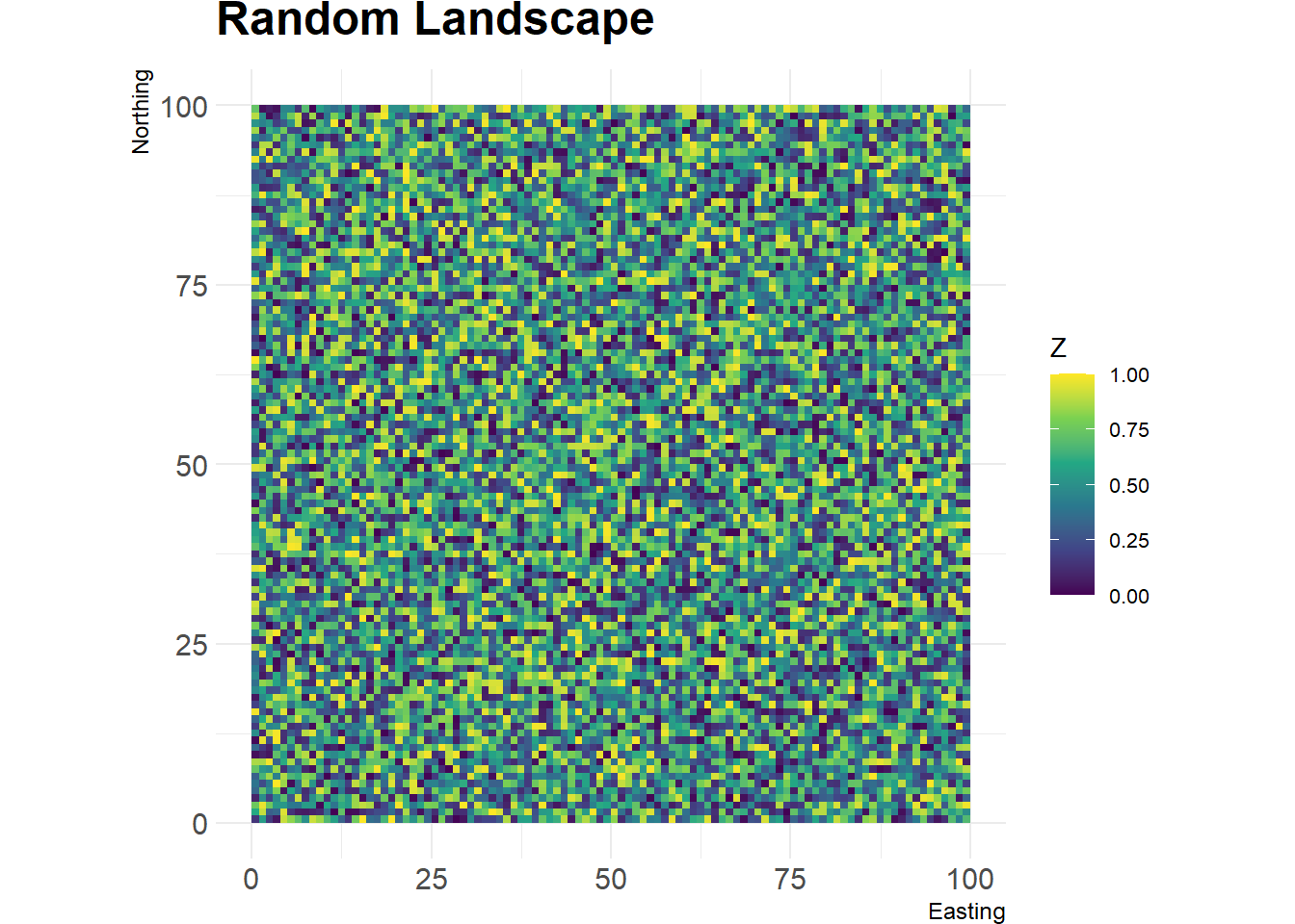
library(gridExtra)10.1 Random
- Random landscape raster drawn from a uniform distribution from 0 to 1
Null baseline for comparing spatial structure to
Simulating the influence of random disturbances or habitat patterns
10.2 Gradient
- Planar gradient landscape raster drawn. Direction of gradient is random by default or can be set manually in degrees as I have here. Useful for modeling environmental gradients like elevation or temperature. You can also do an edge gradient where the peak is in the center of the raster.
nlm2 <- nlm_planargradient(ncol = 100, nrow = 100, direction = 90)
show_landscape(nlm2) + ggtitle("Planar Gradient")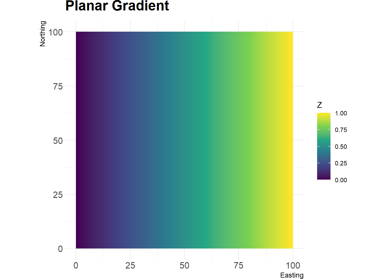
10.3 Mosiac tessellation
- Generates a tesselated landscape. This creates a realistic looking patchy landscape with discrete regions:
nlm3 <- nlm_mosaictess(ncol = 100, nrow = 100, germs = 25)
show_landscape(nlm3) + ggtitle("Mosaic Tessellation")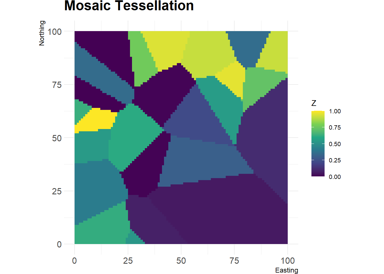
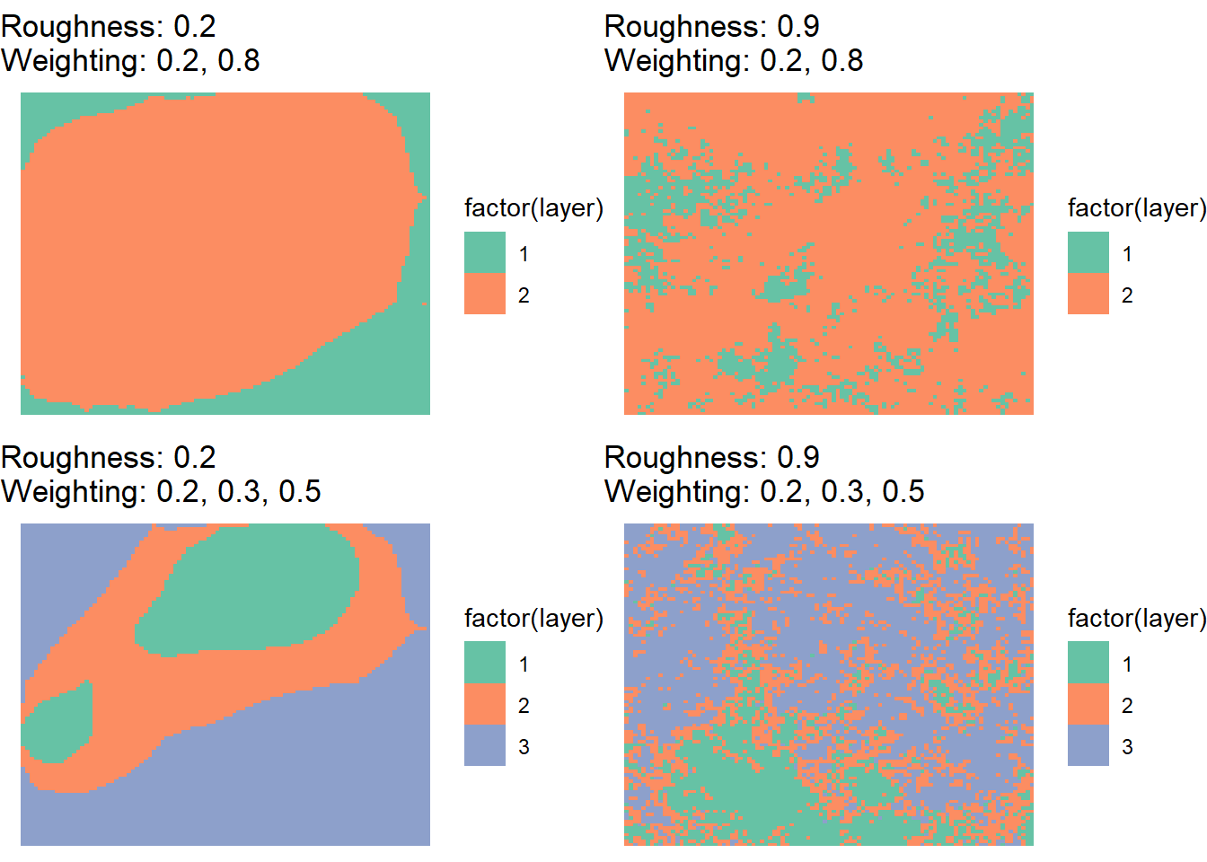
10.4 Simulating across a gradient
- You can also simulate across some parameter values as in some of the ppt examples. This uses yet another simulation called the midpoint displacement neutral landscape model. This is a fractal based algorithm borrowed from generating random terrain in computer graphics/games.
simulate_landscape <- function(roughness, weighting){
  nlm_mpd(ncol = 99,
          nrow = 99,
          roughness = roughness,
          rescale = TRUE) %>%
    util_classify(weighting = weighting)
}

# Parameter combinations
param_df <- expand.grid(
  roughness = c(0.2, 0.9),
  weighting = I(list(c(0.2, 0.8), c(0.2, 0.3, 0.5)))
) %>%
  as_tibble()

# Generate landscapes
nlm_list <- param_df %>% pmap(simulate_landscape)


# Create individual plots
nlm_plots <- lapply(seq_along(nlm_list), function(i) {
  ggplot() +
    geom_raster(data = rasterToPoints(nlm_list[[i]]) %>% as.data.frame(),
                aes(x = x, y = y, fill = factor(layer))) +
    scale_fill_brewer(palette = "Set2") +
    theme_void() +
    ggtitle(paste("Roughness:", param_df$roughness[i],
                  "\nWeighting:", paste(param_df$weighting[[i]], collapse = ", ")))
})

# Arrange and display in a grid
grid.arrange(grobs = nlm_plots, ncol = 2)