20 文本数据分析
R 语言官网的任务视图中有自然语言处理(Natural Language Processing)视图,它涵盖文本数据分析(Text Analysis)的内容。R 语言社区中有两本文本分析相关的著作,分别是《Text Mining with R》(Silge 和 Robinson 2017)和《Supervised Machine Learning for Text Analysis in R》(Hvitfeldt 和 Silge 2021)。
本文获取 CRAN 上发布的 R 包元数据中的描述字段,利用文本分析工具,实现 R 包主题分类。首先加载后续用到的一些文本分析和建模的 R 包。
接着,调用 tools 包的函数 CRAN_package_db() 获取 R 包元数据,为了方便后续重复使用,保存到本地。
去除重复的记录,保留 Package 和 Title 字段,该数据集共含有 22509 个 R 包的元数据。
#>         Package
#> 1 AalenJohansen
#> 2       aamatch
#> 3      AATtools
#> 4        ABACUS
#> 5   abasequence
#> 6    abbreviate
#>                                                                   Title
#> 1                                 Conditional Aalen-Johansen Estimation
#> 2    Artless Automatic Multivariate Matching for Observational\nStudies
#> 3      Reliability and Scoring Routines for the Approach-Avoidance Task
#> 4 Apps Based Activities for Communicating and Understanding\nStatistics
#> 5                               Coding 'ABA' Patterns for Sequence Data
#> 6                                          Readable String Abbreviation
20.1 语料预处理
- 去掉换行符
\n和单引号',字母全部转小写等。
- 提取词干和词形还原。这一步比较麻烦,需要先使用 spacyr 包解析出词性,再根据词性使用不同的规则处理。做名词还原调用 SemNetCleaner 包的函数
singularize(),如 models / modeling 还原为 model, methods 还原为 method 等等。
#> [1] "method" "model" "data"library(spacyr)
# OpenMP
Sys.setenv(KMP_DUPLICATE_LIB_OK = TRUE)
# 初始化 不需要实体识别
spacy_initialize(model = "en_core_web_sm", entity = F)
# 准备解析文本向量
title_desc <- pdb$Title
names(title_desc) <- pdb$Package
# 解析文本需要一点时间约 1 分钟
title_token <- spacy_parse(x = title_desc, entity = F)
# 调用 data.table 操作数据提升效率
library(data.table)
title_token <- as.data.table(title_token)
# 生成新的一列作为 lemma
title_token$lemma2 <- title_token$lemma
# 处理动词和名词
title_token$lemma2 <- fcase(
title_token$pos %in% c("VERB", "AUX"), title_token$lemma,
title_token$pos %in% c("NOUN", "PROPN", "PRON"), vec_singularize(title_token$token),
!title_token$pos %in% c("VERB", "AUX", "NOUN", "PROPN", "PRON"), title_token$token
)
# 还原成向量
pdb <- aggregate(title_token, lemma2 ~ doc_id, paste, collapse = " ")
colnames(pdb) <- c("Package", "Title")
# 清理中间变量
rm(title_token, title_desc)R 包标题文本的长度分布
代码

接下来,要把该数据集整理成文本分析工具可以使用的数据类型 – 制作语料。
20.2 关键词检索
关键词检索就是从语料中查询某个字词及其在语料中的位置,函数 kwic() (函数名是 keywords-in-context 简写)用来做这个事。举两个例子,第一个例子查询语料中包含 Stan 的条目且精确匹配,返回检索词前后 3 个词。第二个例子查询语料中包含 text mining 的条目,采用正则方式匹配,返回检索词前后 2 个词。
#> Keyword-in-context with 38 matches.
#>           [bayesdfa, 6]           factor analysis dfa | stan |
#>      [bayesforecast, 5]             time series model | stan |
#>          [BayesGmed, 6]        mediation analysis use | stan |
#>            [bayesvl, 9]          network perform mcmc | stan |
#>            [blmeco, 13]                     use r bug | stan |
#>           [bmscstan, 7]                case model use | stan |
#>               [bnns, 4]       bayesian neural network | stan |
#>     [breathteststan, 1]                               | stan |
#>               [brms, 5]          regression model use | stan |
#>              [CARME, 4]              car mm modelling | stan |
#>             [edstan, 1]                               | stan |
#>            [flocker, 4] flexible occupancy estimation | stan |
#>        [gptoolsStan, 5]         process graph lattice | stan |
#>  [greencrab.toolkit, 2]                           run | stan |
#>              [hbamr, 7]          mckelvey scaling via | stan |
#>            [hbsaems, 8]          estimation model use | stan |
#>             [hsstan, 3]        hierarchical shrinkage | stan |
#>              [measr, 5]  psychometric measurement use | stan |
#>           [MetaStan, 5]             meta analysis via | stan |
#>               [mlts, 7]                series model r | stan |
#>       [pcFactorStan, 1]                               | stan |
#>              [prome, 6]         outcome data analysis | stan |
#>              [rstan, 3]                   r interface | stan |
#>           [rstanarm, 6]          regression model via | stan |
#>          [rstanemax, 4]           emax model analysis | stan |
#>         [rstantools, 6]           r package interface | stan |
#>           [RStanTVA, 3]                     tva model | stan |
#>       [ssMousetrack, 9]          track experiment via | stan |
#>          [stan4bart, 5]      additive regression tree | stan |
#>        [StanHeaders, 4]                 c header file | stan |
#>         [staninside, 3]                facilitate use | stan |
#>           [StanMoMo, 4]  bayesian mortality modelling | stan |
#>           [survstan, 6]          regression model via | stan |
#>           [tdcmStan, 3]             automate creation | stan |
#>            [tmbstan, 7]              model object use | stan |
#>               [trps, 6]            position model use | stan |
#>     [truncnormbayes, 7]       normal distribution use | stan |
#>               [ubms, 7]           unmarked animal use | stan |
#>
#>
#>
#>
#>
#>
#>
#>
#>  base fit gastric
#>
#>
#>  model item response
#>
#>
#>  model interpret green
#>
#>
#>  model biomarker selection
#>
#>
#>
#>  model pair comparison
#>
#>
#>
#>
#>
#>  use r stantva
#>
#>  sample parametric extension
#>
#>  within package
#>
#>
#>  code tdcms
#>
#>
#>
#> #> Keyword-in-context with 19 matches.
#> [MadanText, 2:3] persian | text mining |
#> [MadanTextNetwork, 2:3] persian | text mining |
#> [malaytextr, 1:2] | text mining |
#> [miRetrieve, 2:3] mirna | text mining |
#> [pubmed.mineR, 1:2] | text mining |
#> [PubMedMining, 1:2] | text mining |
#> [RcmdrPlugin.temis, 3:4] graphical integrate | text mining |
#> [text2vec, 2:3] modern | text mining |
#> [textmineR, 2:3] function | text mining |
#> [TextMiningGUI, 1:2] | text mining |
#> [tidytext, 1:2] | text mining |
#> [tm, 1:2] | text mining |
#> [tm.plugin.alceste, 8:9] use tm | text mining |
#> [tm.plugin.dc, 1:2] | text mining |
#> [tm.plugin.europresse, 6:7] use tm | text mining |
#> [tm.plugin.factiva, 6:7] use tm | text mining |
#> [tm.plugin.lexisnexis, 6:7] use tm | text mining |
#> [tm.plugin.mail, 1:2] | text mining |
#> [tmcn, 1:2] | text mining |
#>
#> tool frequency
#> tool co
#> bahasa malaysia
#> abstract
#> pubmed abstract
#> pubmed repository
#> solution
#> framework r
#> topic modeling
#> gui interface
#> use dplyr
#> package
#> framework
#> distribute corpus
#> framework
#> framework
#> framework
#> e mail
#> toolkit chinese20.3 高频词、词云
发现一些高频出现的词语或短语,通过这些高频词,这暗示一些信息。
#>          data         model      analysis             r           use
#>          3730          2756          2306          1407          1235
#>      function    regression          base          tool    estimation
#>           979           946           919           853           839
#>          test        method          time      bayesian  distribution
#>           745           744           741           688           585
#>     interface           api       network       package        linear
#>           548           539           527           503           496
#>          plot     algorithm        series     inference  multivariate
#>           459           442           417           411           402
#>   statistical        design      multiple      variable        effect
#>           387           381           363           360           350
#>      estimate       spatial          file       cluster     selection
#>           344           341           341           341           338
#>        create     statistic         shiny        sample       dataset
#>           335           326           320           317           305
#>      modeling       process        random           set           via
#>           287           286           275           273           270
#>    simulation visualization          high        robust         value
#>           267           266           262           260           257
R 语言作为一门主要用于数据获取、分析、处理、建模和可视化的统计语言,从 data、analysis、 model 和 regression 等这些高频词可以看出 R 语言面向的领域的特点。在文本分析领域,词云图是很常见的,用来展示文本中的突出信息。下图展示了词频不小于 100 的词。

20.4 关联词、短语
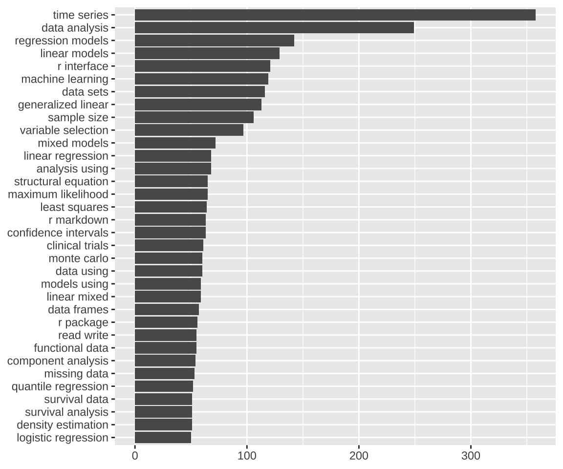
函数 textstat_collocations() 可以挖掘出词与词之间的关联度,下面统计出关联度很高的2个词的情况。
library(quanteda.textstats)
# 2个词 最少出现 50 次
word2 <- pdb_toks |>
  tokens_select(
    pattern = "^[aA-zZ]", valuetype = "regex",
    case_insensitive = FALSE, padding = TRUE
  ) |>
  textstat_collocations(min_count = 50, size = 2, tolower = FALSE)
word2 |>
  subset(select = c("collocation", "count", "lambda", "z")) |>
  (\(x) x[order(x$count, decreasing = T), ])()
#> collocation count lambda z
#> 2 time series 390 8.410134 40.956545
#> 28 data analysis 249 1.917748 26.874453
#> 17 regression model 188 2.766641 31.206371
#> 1 high dimensional 173 8.256046 42.834939
#> 18 linear model 169 3.017284 31.147086
#> 16 data set 133 4.047101 31.276544
#> 26 meta analysis 125 4.912157 27.921690
#> 8 r interface 122 4.243407 35.516868
#> 3 sample size 111 7.215395 38.686341
#> 24 r package 98 3.396362 28.688433
#> 4 variable selection 97 5.472292 38.393389
#> 30 mixed model 96 3.298482 24.518502
#> 5 clinical trial 89 7.381455 37.078679
#> 10 confidence interval 89 7.983490 34.316566
#> 6 single cell 87 7.547635 36.808078
#> 22 least square 80 9.510684 29.199526
#> 7 machine learning 79 6.948648 36.540038
#> 45 analysis use 79 1.648730 13.813474
#> 33 linear regression 75 3.051243 23.510536
#> 43 data frame 75 6.317928 15.432733
#> 27 shiny app 74 8.132907 27.241296
#> 9 change point 73 7.203440 34.899773
#> 44 model base 72 1.823293 14.534360
#> 47 model use 70 1.512122 12.015240
#> 19 linear mixed 69 4.762209 30.695603
#> 23 principal component 69 8.611448 28.988080
#> 14 maximum likelihood 67 7.764512 32.123544
#> 39 effect model 67 2.519713 17.778816
#> 11 structural equation 66 7.194933 34.159026
#> 37 mixture model 66 2.906924 19.287433
#> 50 data use 66 1.027935 8.018226
#> 12 shiny application 65 6.124465 33.816839
#> 15 mixed effect 65 4.951229 31.357782
#> 40 neural network 65 7.937305 17.770993
#> 13 random forest 64 6.038883 32.700797
#> 21 generalize linear 64 4.578363 29.573412
#> 32 r markdown 64 5.654212 23.591816
#> 36 component analysis 64 3.960064 21.671622
#> 49 monte carlo 63 17.035933 8.501237
#> 48 goodness fit 59 12.225399 8.571668
#> 25 read write 58 7.882096 27.925273
#> 38 markov model 56 3.340163 18.865384
#> 42 functional data 55 2.577275 15.733731
#> 20 gaussian process 54 5.558851 30.695369
#> 31 quantile regression 54 4.369405 24.381027
#> 29 density estimation 52 4.516663 25.231081
#> 35 logistic regression 51 5.009119 23.375485
#> 41 survival analysis 51 2.605927 16.294877
#> 46 survival data 51 2.093798 13.141149
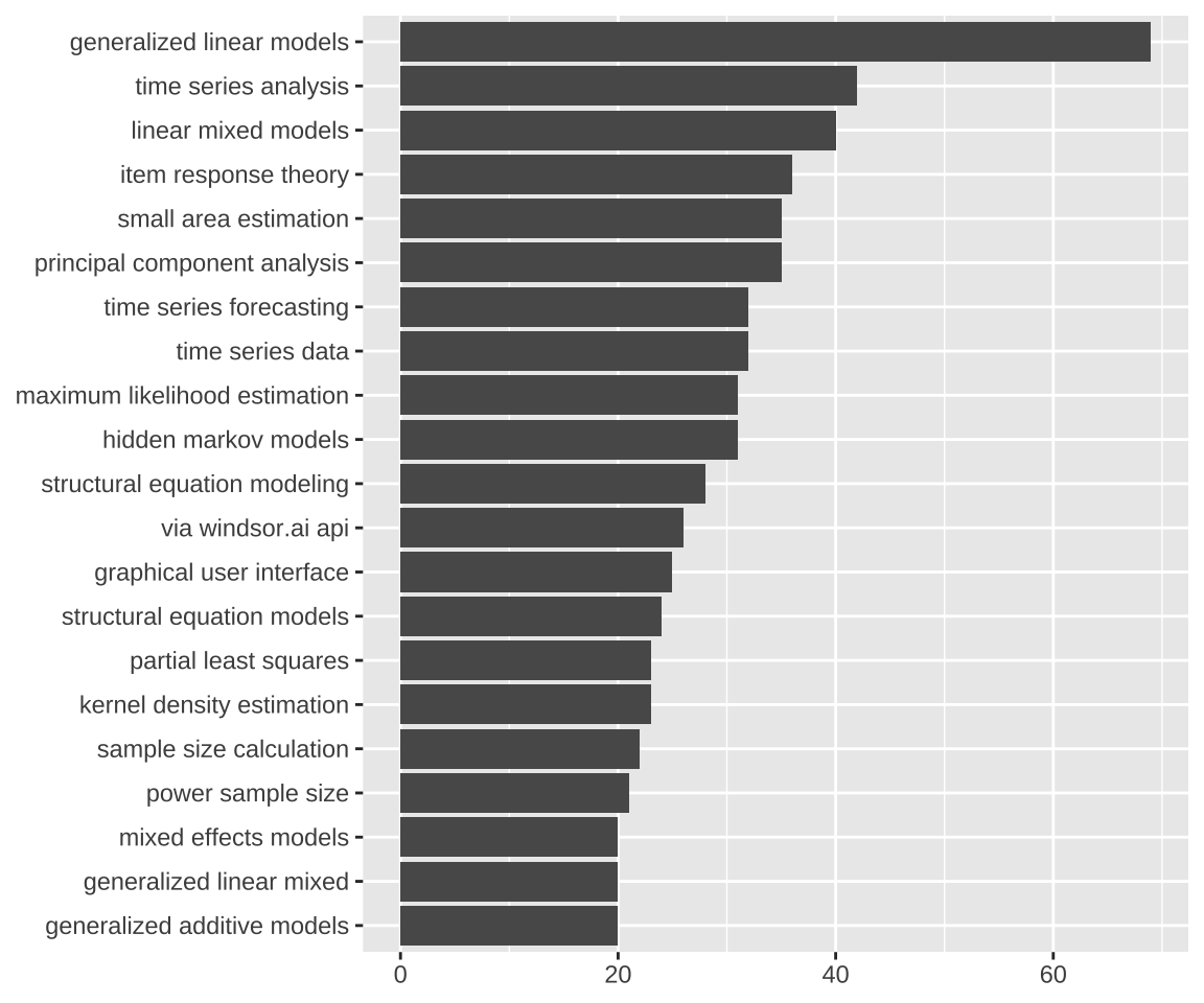
#> 34 utility function 50 4.031428 23.406819下面统计出关联度很高的3个词的情况。
# 3 个词 最少出现 20 次
word3 <- pdb_toks |>
  tokens_select(
    pattern = "^[aA-zZ]", valuetype = "regex",
    case_insensitive = FALSE, padding = TRUE
  ) |>
  textstat_collocations(min_count = 20, size = 3, tolower = FALSE)
word3 |>
  subset(select = c("collocation", "count", "lambda", "z")) |>
  (\(x) x[order(x$count, decreasing = T), ])()
#> collocation count lambda z
#> 1 mixed effect model 52 2.74933933 5.26421311
#> 16 linear mixed model 51 0.29724376 0.79122768
#> 15 time series analysis 44 1.22245001 0.82987380
#> 29 principal component analysis 43 -1.14777702 -1.43212297
#> 8 generalized linear model 41 0.86637873 1.61224892
#> 13 high dimensional data 40 1.11204011 1.20333574
#> 14 change point detection 38 1.80608692 1.14096970
#> 30 generalize linear model 38 -0.83256107 -2.43034663
#> 4 small area estimation 37 3.80872471 2.19968436
#> 6 item response theory 37 3.56746831 1.74474274
#> 27 time series data 35 -0.64298804 -0.72305884
#> 23 goodness fit test 34 0.05365225 0.02171631
#> 21 maximum likelihood estimation 32 0.51772646 0.35048085
#> 12 structural equation model 31 0.92777932 1.24716444
#> 18 sample size calculation 31 0.72939612 0.43875914
#> 3 model base clustering 26 4.66999216 3.16260592
#> 19 via windsor.ai api 26 0.91318357 0.41485214
#> 26 partial least square 26 -0.61192195 -0.29897908
#> 5 graphical user interface 25 4.09997307 1.98995699
#> 7 network meta analysis 25 2.49751077 1.68333680
#> 24 time series forecast 25 -0.07179827 -0.03534369
#> 11 structural equation modeling 24 2.57880356 1.27148555
#> 9 hide markov model 23 2.36565975 1.37903147
#> 20 kernel density estimation 23 0.31263525 0.39090311
#> 10 power sample size 22 2.64371045 1.30480977
#> 17 time series model 22 1.03679417 0.69749215
#> 28 genome wide association 22 -2.05849808 -1.17948789
#> 25 generalize additive model 21 -0.08469047 -0.16409359
#> 2 large language model 20 7.38549608 3.58810691
#> 22 amazon web service 20 0.30375485 0.14705747
#> 31 linear regression model 20 -1.64473425 -4.90001486其中有两个词组 via windsor.ai api 和 amazon web service 乍一看有点奇怪,其实是这两个公司发布的一系列 R 包导致。
代码
20.5 特征共现网络
在文档 Token 化之后,函数 dfm() 构建文档特征(词)矩阵,函数 topfeatures() 提取文档-词矩阵中的主要特征(词)。
#>       data      model   analysis          r        use   function regression
#>       3730       2756       2306       1407       1235        979        946
#>       base       tool estimation
#>        919        853        839
在文档 Token 化之后,函数 fcm() 构建特征(词)共现矩阵,统计词频,挑选前 30 个高频词。
下图以网络图方式展示词与词之间的关联度,关联度越高,词与词之间的边越宽。

20.6 词频文档统计
TF-IDF 词频与逆文档频率(term frequency-inverse document frequency weighting)
#> Document-feature matrix of: 6 documents, 6 features (83.33% sparse) and 0 docvars.
#>                features
#> docs             artless automatic multivariate matching observational    study
#>   AalenJohansen 0          0          0         0             0        0
#>   aamatch       2.409702   1.35011    0.9696616 1.417336      1.473917 1.115005
#>   AATtools      0          0          0         0             0        0
#>   ABACUS        0          0          0         0             0        0
#>   abasequence   0          0          0         0             0        0
#>   abbreviate    0          0          0         0             0        0
每个特征的文档频率
#>       artless     automatic  multivariate      matching observational
#>             1            82           399            62            49
#>         study   reliability       scoring       routine      approach
#>           218            41            22            43           120
#>     avoidance
#>             1
特征频次作为权重
#> Document-feature matrix of: 6 documents, 6 features (83.33% sparse) and 0 docvars.
#>                features
#> docs            artless automatic multivariate matching observational study
#>   AalenJohansen       0         0            0        0             0     0
#>   aamatch             1         1            1        1             1     1
#>   AATtools            0         0            0        0             0     0
#>   ABACUS              0         0            0        0             0     0
#>   abasequence         0         0            0        0             0     0
#>   abbreviate          0         0            0        0             0     0
20.7 潜在语义分析
文档特征矩阵通过 SVD 分解将高维特征(15K)降至低维(10),获得文档主题矩阵与主题特征矩阵两个低秩矩阵,SVD 分解的作用在于去掉大量的噪声,取主要的信号部分(特征值非零的矩阵块)。
#>                        [,1]          [,2]          [,3]          [,4]
#> AalenJohansen -0.0032241844  0.0034427122  1.173770e-03 -0.0048326840
#> aamatch       -0.0016668871 -0.0001994336 -1.901995e-03 -0.0003041840
#> AATtools      -0.0005909884  0.0003214012  5.347647e-05 -0.0004353074
#> ABACUS        -0.0024507910 -0.0009244992  1.526391e-03  0.0038587327
#> abasequence   -0.0234527009 -0.0406546808  2.051835e-02 -0.0177373890
#> abbreviate     0.0000000000  0.0000000000  0.000000e+00  0.0000000000
#>                        [,5]          [,6]         [,7]         [,8]
#> AalenJohansen  0.0022601292 -2.045532e-03  0.001946985 -0.008157300
#> aamatch       -0.0013131362  1.872377e-03 -0.001403527 -0.001269297
#> AATtools       0.0004311038  3.435035e-06 -0.000511839 -0.002978224
#> ABACUS         0.0040831942  2.645468e-03  0.004626168 -0.004909116
#> abasequence   -0.0039105882  2.355800e-03 -0.003129303  0.005084495
#> abbreviate     0.0000000000  0.000000e+00  0.000000000  0.000000000
#>                        [,9]         [,10]
#> AalenJohansen -0.0213592856  0.0544385396
#> aamatch       -0.0046593155  0.0099661478
#> AATtools      -0.0001883452  0.0005746988
#> ABACUS        -0.0143708312  0.0135888747
#> abasequence    0.0004201955 -0.0036880802
#> abbreviate 0.0000000000 0.0000000000#> 10 x 2 Matrix of class "dgeMatrix"
#>
#> docs [,1] [,2]
#> BSGW -0.059292835 0.0519053918
#> bshazard -0.002673471 -0.0012577308
#> bSi -0.001556967 0.0001918223
#> bsicons -0.001247856 -0.0010822795
#> bSims -0.002837332 -0.0005650347
#> bsitar -0.042127715 0.0125912510
#> bskyr 0.000000000 0.0000000000
#> BSL -0.025798774 0.0244089229
#> bslib -0.001122917 -0.0009895321
#> BsMD -0.019458772 0.022141242320.8 文本主题探索
text2vec 包的实现 LDA(Latent Dirichlet Allocation)算法做文本主题建模。
library(text2vec)
# 创建 Tokens
pdb_tokens <- word_tokenizer(pdb$Title)
pdb_itokens <- itoken(pdb_tokens, ids = pdb$Package, progressbar = FALSE)
# 去掉停止词
pdb_v <- create_vocabulary(pdb_itokens, stopwords = stopwords("en"))
# 词频不小于 10 的词
# 文档比例不大于 0.2
pdb_v <- prune_vocabulary(pdb_v, term_count_min = 10, doc_proportion_max = 0.2)
pdb_v
#> Number of docs: 22509
#> 175 stopwords: i, me, my, myself, we, our ...
#> ngram_min = 1; ngram_max = 1
#> Vocabulary:
#> term term_count doc_count
#> <char> <int> <int>
#> 1: 2019 10 7
#> 2: 4 10 10
#> 3: account 10 10
#> 4: active 10 10
#> 5: allow 10 10
#> ---
#> 1671: use 1235 1235
#> 1672: r 1408 1388
#> 1673: analysis 2306 2288
#> 1674: model 2756 2687
#> 1675: data 3730 3634vectorizer <- vocab_vectorizer(pdb_v)
pdb_dtm <- create_dtm(pdb_itokens, vectorizer, type = "dgTMatrix")
lda_model <- LDA$new(n_topics = 10, doc_topic_prior = 0.1, topic_word_prior = 0.01)
doc_topic_distr <- lda_model$fit_transform(
x = pdb_dtm, n_iter = 1000,
convergence_tol = 0.001, n_check_convergence = 25,
progressbar = FALSE
)代码
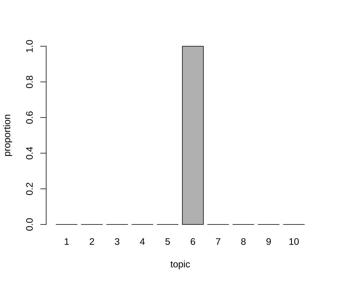
每个主题抽取 Top 的 10 个词
#>       [,1]       [,2]            [,3]           [,4]         [,5]
#>  [1,] "time"     "data"          "model"        "regression" "data"
#>  [2,] "model"    "plot"          "linear"       "model"      "analysis"
#>  [3,] "series"   "tool"          "bayesian"     "variable"   "use"
#>  [4,] "analysis" "ggplot2"       "data"         "selection"  "association"
#>  [5,] "learning" "use"           "distribution" "algorithm"  "calculate"
#>  [6,] "machine"  "analysis"      "mixed"        "linear"     "population"
#>  [7,] "base"     "visualization" "mixture"      "estimation" "estimate"
#>  [8,] "response" "function"      "regression"   "use"        "quality"
#>  [9,] "function" "map"           "analysis"     "method"     "control"
#> [10,] "learn"    "set"           "generalize"   "base"       "base"
#>       [,6]          [,7]        [,8]          [,9]           [,10]
#>  [1,] "data"        "r"         "test"        "estimation"   "r"
#>  [2,] "analysis"    "data"      "sample"      "model"        "function"
#>  [3,] "design"      "api"       "analysis"    "data"         "shiny"
#>  [4,] "tool"        "interface" "base"        "regression"   "package"
#>  [5,] "trial"       "access"    "two"         "distribution" "use"
#>  [6,] "network"     "file"      "size"        "high"         "application"
#>  [7,] "cell"        "package"   "measure"     "dimensional"  "create"
#>  [8,] "single"      "database"  "correlation" "analysis"     "file"
#>  [9,] "clinical"    "client"    "power"       "test"         "table"
#> [10,] "statistical" "wrapper"   "value"       "robust"       "data"
TODO: 使用交叉验证配合 perplexity 度量获取最佳的主题个数 (Zhang, Li, 和 Zhang 2023)
20.9 文本相似性
在互联网 App 中,计算文本之间的相似性有很多应用,如搜索、推荐和广告的召回阶段,根据用户输入的文本召回相关的内容。
text2vec 包实现了 GloVe 模型 — 一种词向量表示的无监督学习算法。从语料中生成词共现矩阵,基于此训练数据,算法得出的是词向量空间中的线性子结构。GloVe 度量了词与词之间共现的可能性,词与词抽象的概念差异可以表示成向量的差异。下面继续基于这份文本数据,生成词共现矩阵,计算文本相似度。
参考 quanteda 包官网对 text2vec 包GloVe 模块的介绍。
GloVe 模型
#> [1] 2747 50#> [1] 50 2747计算距离
cpp <- word_vectors["rcpp", , drop = FALSE] -
  word_vectors["stan", , drop = FALSE] +
    word_vectors["python", , drop = FALSE]

# 文档的余弦相似性 取一个小数据
library(quanteda.textstats)
cos_sim <- textstat_simil(
  x = as.dfm(word_vectors), y = as.dfm(cpp),
  margin = "documents", method = "cosine")
# 召回的相关词
head(sort(cos_sim[, 1], decreasing = TRUE), 5)
#> rcpp python integration smith binding
#> 0.7009370 0.6591426 0.5411046 0.4424318 0.417090720.10 习题
text2vec 包内置的电影评论数据集
movie_review中 sentiment(表示正面或负面评价)列作为响应变量,构建二分类模型,对用户的一段评论分类。(提示:词向量化后,采用 glmnet 包做交叉验证调整参数、模型)根据任务视图对 R 包的标记,建立有监督的多分类模型,评估模型的分类效果,并对尚未标记的 R 包分类。(提示:一个 R 包可能同时属于多个任务视图,考虑使用 xgboost 包)