1 When \(y\) is continuous: general linear model

The term “general” linear model (GLM) usually refers to conventional linear regression models for a continuous response variable given continuous and/or categorical predictors. It includes multiple linear regression, as well as ANOVA and ANCOVA (with fixed effects only).

1.1 When \(x\) is continuous

For simplicity, multiple regression in this chapter is referring to multiple regression with fixed \(x\).

\[y_i=\beta_0+\beta_1x_{1i}+\cdots+\beta_px_{pi}+\epsilon_i,\] In the model above, we assume that \(\epsilon_i\) and \(y_i\) are random variables, \(x_i\)s are known constants. we have several assumptions:

\(E(\epsilon_i)=0\), or equivalently, \(E(y_i)=\beta_0+\beta_1x_i\);
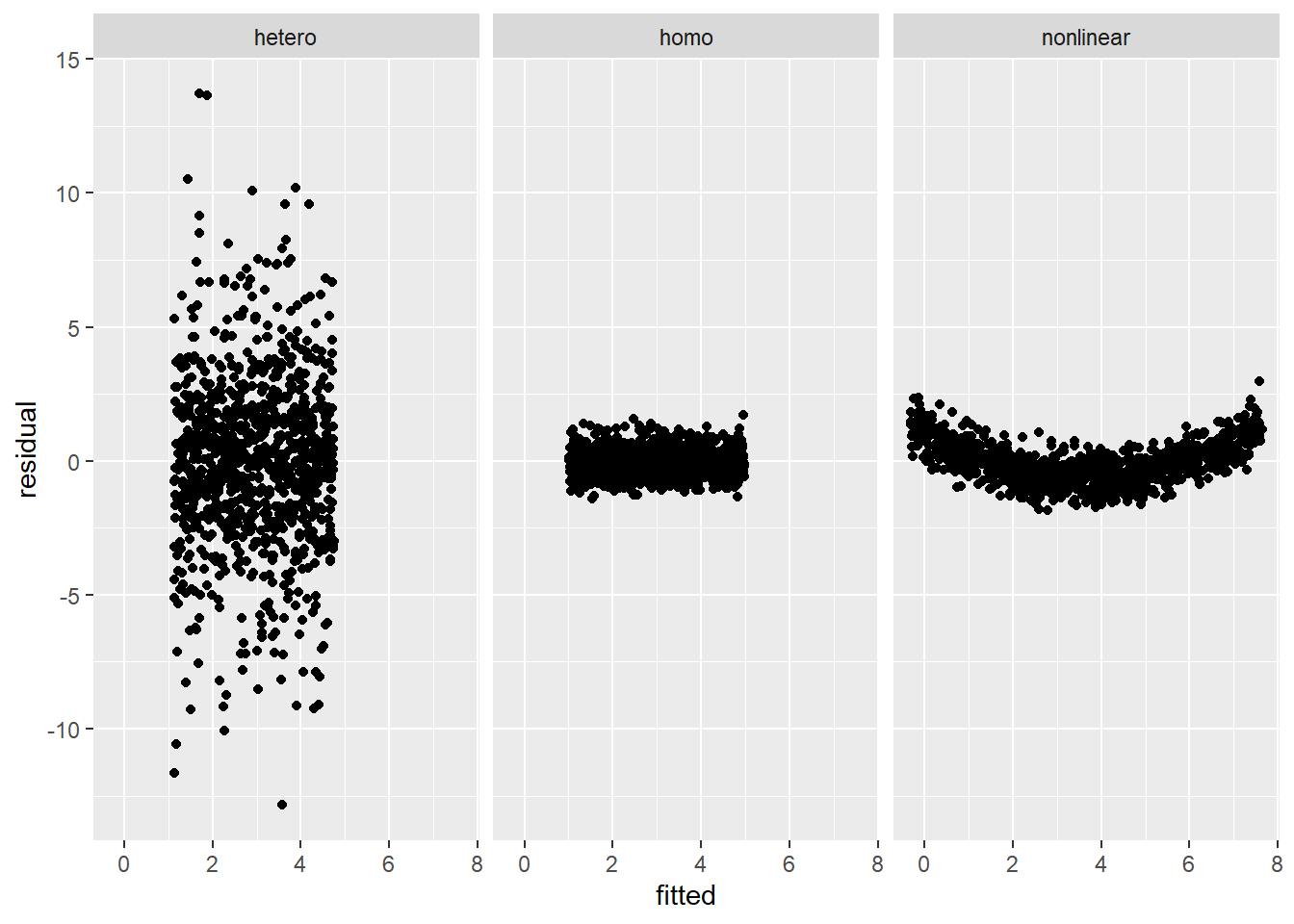
\(\text{var}(\epsilon_i)=\sigma^2\), or equivalently, \(\text{var}(y_i)=\sigma^2\);
\(\text{cov}(\epsilon_i,\epsilon_j)=0\) for all \(i\neq j\), or, equivalently, \(\text{cov}(y_i, y_j)=0\).

Assumption 1 states that the value of \(y_i\) depends on all \(x_i\)s, all other variation in \(y_i\) is random error.

Assumption 2 states that \(\epsilon_i\)s have identical variance. This is also known as the assumption of homoscedasticity, homogeneous variance or constant variance.

After fitting a multiple regression model to a given data set we shall have \[\hat{y}_i=\hat{\beta}_0+\hat{\beta}_1x_{1i}+\cdots+\hat{\beta}_px_{pi}\] where \(\hat{\beta}_0\) and \(\hat{\beta}_j\) are the corresponding estimated intercept and slope, \(\hat{y}_i\) is the predicted \(y\) of \(x_{1i},\cdots,x_{pi}\) by the model above.

1.1.1 How to generate data using multiple regression

Simple regression

Generate a set of data that satisfy \(y = 1 + x_1+\epsilon\).

set.seed(123)
n <- 300
beta_0 <- 1
beta_1 <- 1
x1 <- 1:n
epsilon <- rnorm(n, mean = 0, sd = 1)
y <- beta_0 + beta_1*x1 + epsilon
df <- data.frame(x1 = x1, y = y)
model_1 <- lm(y ~ x1, data = df)
summary(model_1)

#> 
#> Call:
#> lm(formula = y ~ x1, data = df)
#> 
#> Residuals:
#>     Min      1Q  Median      3Q     Max 
#> -2.3053 -0.6368 -0.0705  0.5928  3.2000 
#> 
#> Coefficients:
#>              Estimate Std. Error  t value Pr(>|t|)    
#> (Intercept) 0.9610022  0.1095565    8.772   <2e-16 ***
#> x1          1.0004880  0.0006309 1585.691   <2e-16 ***
#> ---
#> Signif. codes:  0 '***' 0.001 '**' 0.01 '*' 0.05 '.' 0.1 ' ' 1
#> 
#> Residual standard error: 0.9464 on 298 degrees of freedom
#> Multiple R-squared:  0.9999, Adjusted R-squared:  0.9999 
#> F-statistic: 2.514e+06 on 1 and 298 DF,  p-value: < 2.2e-16

coef(model_1)

#> (Intercept)          x1 
#>   0.9610022   1.0004880

Multiple regression

Generate a set of data that satisfy \(y = 1 + 2x_1 + 3x_2+\epsilon\)

set.seed(123)
n <- 300
beta_0 <- 1
beta_1 <- 2
beta_2 <- 3
x1 <- 1:300
x2 <- sample(n, n)
epsilon <- rnorm(n, mean = 0, sd = 1)
y <- beta_0 + beta_1*x1 + beta_2*x2 + epsilon
df <- data.frame(x1 = x1, x2 = x2, y = y)
model_1 <- lm(y ~ x1 + x2, data = df)
summary(model_1)

#> 
#> Call:
#> lm(formula = y ~ x1 + x2, data = df)
#> 
#> Residuals:
#>      Min       1Q   Median       3Q      Max 
#> -2.64350 -0.62079  0.00596  0.68103  2.48339 
#> 
#> Coefficients:
#>              Estimate Std. Error  t value Pr(>|t|)    
#> (Intercept) 1.1094805  0.1474924    7.522 6.44e-13 ***
#> x1          1.9999022  0.0006593 3033.340  < 2e-16 ***
#> x2          2.9996187  0.0006593 4549.654  < 2e-16 ***
#> ---
#> Signif. codes:  0 '***' 0.001 '**' 0.01 '*' 0.05 '.' 0.1 ' ' 1
#> 
#> Residual standard error: 0.9872 on 297 degrees of freedom
#> Multiple R-squared:      1,  Adjusted R-squared:      1 
#> F-statistic: 1.584e+07 on 2 and 297 DF,  p-value: < 2.2e-16

1.1.2 Intuitive understanding of ordinary least square

Suppose we have \(y=\hat{a}x\), where \(a\) is parameter yet-to-estimate, \(x\) and \(y\) are observed variables. The straightforward estimator would be moving \(x\) to the left hand side by division \(\hat{a}=y/x\).

Similarly, given the matrix representation of multiple linear regression \(\boldsymbol{y}=\boldsymbol{X}\hat{\boldsymbol{\beta}}\), the simplest solution to derive the formula of \(\hat{\boldsymbol{\beta}}\) would be dividing \(\boldsymbol{y}\) by \(\boldsymbol{X}\), the operation corresponding to division in linear algebra is inversion. However, only square matrix with full rank is invertible. How to construct an invertible square matrix based on \(\boldsymbol{X}\)? \[\begin{align*} \boldsymbol{X}'y&=\boldsymbol{X}'\boldsymbol{X}\hat{\boldsymbol{\beta}}\\ (\boldsymbol{X}'\boldsymbol{X})^{-1}\boldsymbol{X}'y&=\hat{\boldsymbol{\beta}}. \end{align*}\]

# OLS by hand
set.seed(123)
n <- 300
beta_0 <- 1
beta_1 <- 2
beta_2 <- 3
x1 <- 1:300
x2 <- sample(n, n)
epsilon <- rnorm(n, mean = 0, sd = 1)
y <- beta_0 + beta_1*x1 + beta_2*x2 + epsilon
df <- data.frame(x1 = x1, x2 = x2, y = y)
model_1 <- lm(y ~ x1 + x2, data = df)
summary(model_1)

#> 
#> Call:
#> lm(formula = y ~ x1 + x2, data = df)
#> 
#> Residuals:
#>      Min       1Q   Median       3Q      Max 
#> -2.64350 -0.62079  0.00596  0.68103  2.48339 
#> 
#> Coefficients:
#>              Estimate Std. Error  t value Pr(>|t|)    
#> (Intercept) 1.1094805  0.1474924    7.522 6.44e-13 ***
#> x1          1.9999022  0.0006593 3033.340  < 2e-16 ***
#> x2          2.9996187  0.0006593 4549.654  < 2e-16 ***
#> ---
#> Signif. codes:  0 '***' 0.001 '**' 0.01 '*' 0.05 '.' 0.1 ' ' 1
#> 
#> Residual standard error: 0.9872 on 297 degrees of freedom
#> Multiple R-squared:      1,  Adjusted R-squared:      1 
#> F-statistic: 1.584e+07 on 2 and 297 DF,  p-value: < 2.2e-16

# least square
xs <- cbind(1, x1, x2)
y <- as.matrix(y)
beta_byhand <- solve(t(xs) %*% xs) %*% t(xs) %*% y
beta_byhand

#>        [,1]
#>    1.109481
#> x1 1.999902
#> x2 2.999619

1.1.3 A few caveats

\(x\) is fixed

we assume that \(y_i\) and \(\epsilon_i\) are random variables and that the values of \(x_i\) are known constants, which means that the same values of \(x_1, x_2, \ldots, x_n\) would be used in repeated sampling

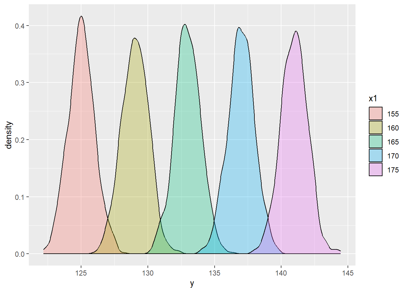
# predict the height of child by the average height of parents
set.seed(123)
n_child_per_height <- 1000
beta_0 <- 1
beta_1 <- 0.8
height_ave_parents <- rep(
  seq(155, 175, by = 5), 
  each = n_child_per_height
)
epsilon <- rnorm(length(height_ave_parents), mean = 0, sd = 1)
y <- beta_0 + beta_1*height_ave_parents + epsilon
df <- data.frame(x1 = height_ave_parents, y = y)
model_1 <- lm(y ~ x1, data = df)
df$x1 <- factor(df$x1)
ggplot(df, aes(x = y, fill = x1)) + 
  geom_density(alpha = 0.3)

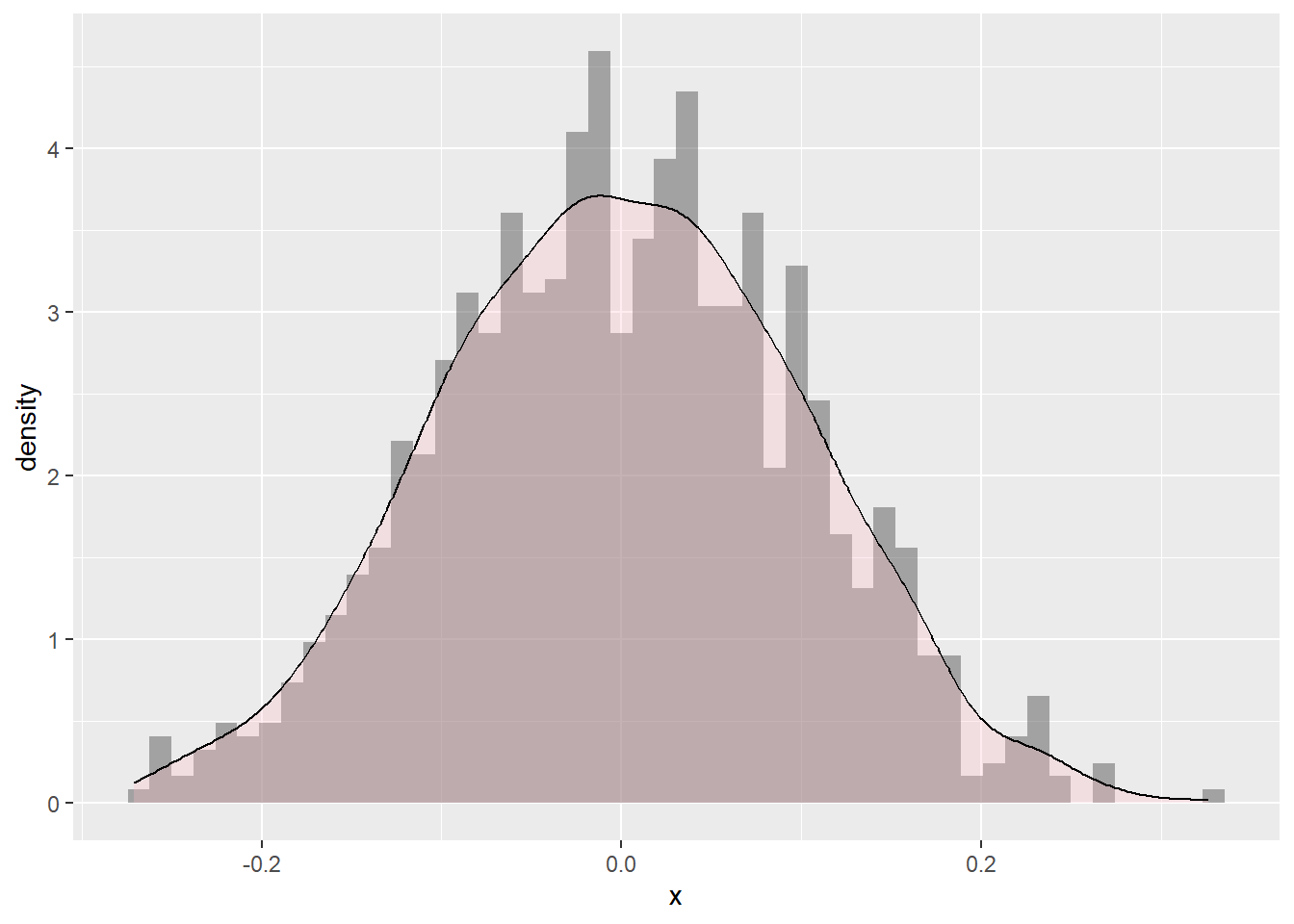
\(\hat{\epsilon}\)s are normally distributed but \(\boldsymbol{y}\) is not

The distribution of \(y\) is not necessarily normal, because

\[y_i \sim N(\beta_0+\beta_1x_{1i}+\cdots+\beta_px_{pi}, \sigma^2),\]

they are all from different normal distributions, their assemblage can be anything.

set.seed(123)
n <- 1000
beta_0 <- 10
beta_1 <- 5
beta_2 <- 1
x1 <- sample(100:105, n, replace = T)
x2 <- 1:n
epsilon <- rnorm(n, mean = 0, sd = 0.1)
y <- beta_0 + beta_1*x1 + beta_2*x2 + epsilon
df <- data.frame(x1 = x1, x2 = x2, y = y)
model_1 <- lm(y ~ x1 + x2, data = df)
hist(y)

df_plot <- data.frame(x = model_1$residuals)
ggplot(df_plot, aes(x = x)) + 
  geom_histogram(aes(y = ..density..), bins = 50, alpha = 0.5) +
  geom_density(fill = "pink", alpha = 0.3)

The interpretation of intercept \(\beta_0\) and slope \(\beta_j\)

Intercept

The intercept \(\beta_0\) could be viewed as the value of \(\hat{y}\) when all \(x\)s equal zero, it is only meaningful if it’s reasonable that all of the predictor variables in the data tested can actually be equal to zero. For example, if we fit a simple regression with height as \(x\) and weight as \(y\), certainly we can estimate a simple regression with intercept, but height equals 0 is make no sense at all. In this case, the intercept term simply anchors the regression line in the right place.

Slope

The slope \(\hat{\beta}_j\) signifies how much \(\hat{y}\) changes given a one-unit shift in \(x_j\) while holding other \(x\)s in the model constant. This property of holding the other independent variables constant is crucial because it allows you to assess the effect of each \(x\) on \(y\) in isolation from the others. If you are familiar with ANOVA, the interpretation of slope is similar to that of simple main effect.

In multiple regression, the relationship between \(x_j\) and \(y\) is linear, implying that the change of y in \(x_j\) is constant (\(\beta_j\) remains unchanged).

set.seed(123)
n <- 300
beta_0 <- 1
beta_1 <- 2
beta_2 <- 3
x1 <- sample(n, n, replace = TRUE)
x2 <- sample(n, n, replace = TRUE)
y <- beta_0 + beta_1*x1 + beta_2*x2 + rnorm(n)
df <- data.frame(x1 = x1, x2 = x2, y = y)
fit <- lm(y ~ x1 + x2, data = df)
coefs <- coef(fit)
coefs

#> (Intercept)          x1          x2 
#>    1.026029    1.999878    2.999837

coefs[1] + 51*coefs[2] + 10*coefs[3] - (coefs[1] + 50*coefs[2] + 10*coefs[3])

#> (Intercept) 
#>    1.999878

coefs[1] + 100*coefs[2] + 10*coefs[3] - (coefs[1] + 99*coefs[2] + 10*coefs[3])

#> (Intercept) 
#>    1.999878

Centering, to make the intercept interpretable

Centering = subtract a constant from each observation so that the 0 value falls within the range of the new centered predictor variable.

Typical: Center around predictor’s mean, i.e. centering \(x\), \(x-\bar{x}\). Intercept is then expected outcome for “average \(x\)”.
Better: Center around meaningful constant \(C\), i.e. centering \(x\), \(x-C\). Intercept is then expected outcome for “\(x=C\)”.

1.1.4 Testing assumptions

1.1.4.1 Independence of \(\epsilon\)s

\[\begin{align*} COV(\boldsymbol{\epsilon})=\begin{bmatrix} \sigma^2 & 0 & 0 & \cdots & 0 \\ 0 & \sigma^2 & 0 & \cdots & 0 \\ \vdots & & & & \vdots\\ 0 & 0 & \cdots & \sigma^2 & 0 \\ 0 & 0 & 0 & \cdots & \sigma^2 \end{bmatrix}=I\sigma^2 \end{align*}\]

set.seed(123)
n <- 1000
beta_0 <- 1
beta_1 <- 2
beta_2 <- 3
x1 <- sample(n, size = n, replace = TRUE)
x2 <- sample(n, size = n, replace = TRUE)
epsilon <- rnorm(n, mean = 0, sd = 1)
y <- beta_0 + beta_1*x1 + beta_2*x2 + epsilon
df <- data.frame(x1 = x1, x2 = x2, y = y)
model_1 <- lm(y ~ x1 + x2, data = df)
# scatter plot
df_plot <- data.frame(
  x = model_1$residuals[-1], 
  y = model_1$residuals[-n]
)
ggplot(df_plot, aes(x = x, y = y)) + 
  geom_point()

car::durbinWatsonTest(model_1)

#>  lag Autocorrelation D-W Statistic p-value
#>    1    -0.002420309      2.003365   0.952
#>  Alternative hypothesis: rho != 0

1.1.4.2 Constant variance

set.seed(123)
n <- 1000
beta_0 <- 1
beta_1 <- 2
x <- runif(n, min = 0, max = 2)
epsilon_homo <- rnorm(n, mean = 0, sd = 0.5)
sds <- seq(1, 5, length.out = 10)
epsilon_hetero <- 
  sapply(sds, \(x) rnorm(100, mean = 0, sd = x)) |> 
  Reduce(f = c, x = _)
y_homo <- beta_0 + beta_1 * x + epsilon_homo
y_hetero <- beta_0 + beta_1 * x + epsilon_hetero
y_nonlinear <- beta_0 + beta_1*x^2 + epsilon_homo
df <- data.frame(
  x = x, 
  y_homo = y_homo, 
  y_hetero = y_hetero, 
  y_nonlinear = y_nonlinear
)
model_homo <- lm(y_homo ~ x, data = df)
model_hetero <- lm(y_hetero ~ x, data = df)
model_nonlinear <- lm(y_nonlinear ~ x, data = df)
data.frame(
  fitted_homo = model_homo$fitted.values,
  residual_homo = model_homo$residuals,
  fitted_hetero = model_hetero$fitted.values,
  residual_hetero = model_hetero$residuals, 
  fitted_nonlinear = model_nonlinear$fitted.values,
  residual_nonlinear = model_nonlinear$residuals
) |> 
  pivot_longer(
    cols = 1:6, 
    names_to = c(".value", "group"), 
    names_sep = "_"
  ) |>
  ggplot(aes(x = fitted, y = residual)) + 
  geom_point() +
  facet_grid(cols = vars(group))

1.1.4.3 Normality

set.seed(123)
n <- 1000
beta_0 <- 1
beta_1 <- 2
beta_2 <- 3
x1 <- sample(n, n, replace = T)
x2 <- sample(n, n, replace = T)
epsilon <- rnorm(n, mean = 0, sd = 1)
y <- beta_0 + beta_1*x1 + beta_2*x2 + epsilon
df <- data.frame(x1 = x1, x2 = x2, y = y)
model_1 <- lm(y ~ x1 + x2, data = df)
df_plot <- data.frame(
  x = model_1$residuals
)
ggplot(df_plot, aes(sample = x)) + 
  stat_qq() + 
  stat_qq_line()

shapiro.test(df_plot$x)

#> 
#>  Shapiro-Wilk normality test
#> 
#> data:  df_plot$x
#> W = 0.99807, p-value = 0.3153

ks.test(df_plot$x, y = "pnorm")

#> 
#>  Asymptotic one-sample Kolmogorov-Smirnov test
#> 
#> data:  df_plot$x
#> D = 0.021975, p-value = 0.7197
#> alternative hypothesis: two-sided

1.2 When \(x\) is categorical

The validity of the interpretation of slope hinges on the interval nature of \(x\), since \(\hat{\beta}_j\) is interpreted as how \(\hat{y}\) would change in one-unit shift of \(x_j\) while holding other independent variables at constant. In other words, the high and low values of \(x\) are meaningful. However, when \(x\) is categorical (ordinal or nominal), the one-unit change of \(x\) becomes meaningless (ordinal variable has no equal intervals, nominal has neither euqal intervals and order), thus we need to use coding scheme, of which the most widely used one is dummy coding.

Dummy Coding: The how and why

The interpretation of regression coefficient with dummy variables

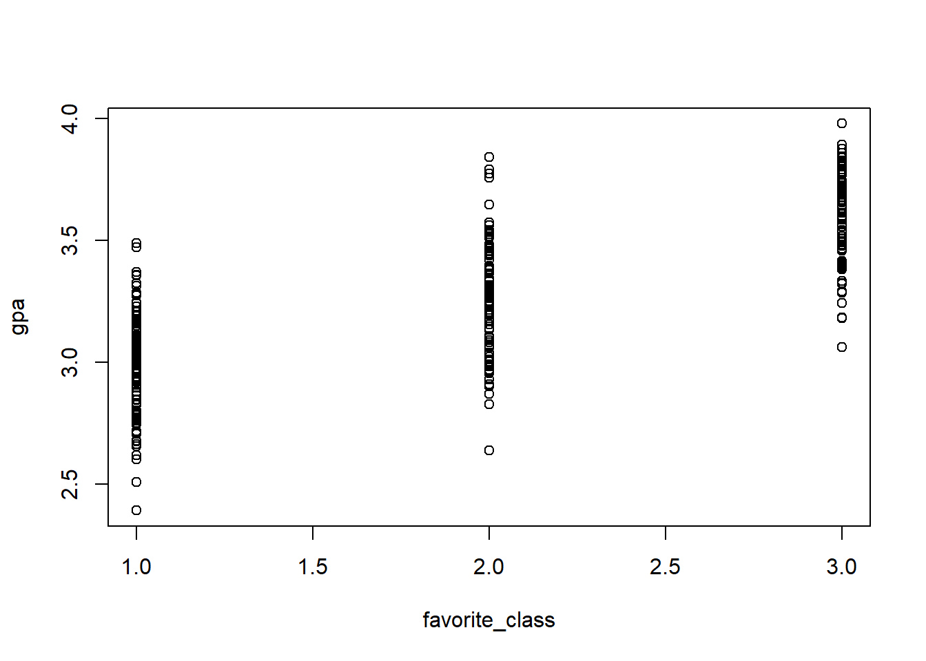
Before dummy coding, the regression model is \[\text{GPA}_i=\beta_0+\beta_1\text{FavoriteClass}_i+\epsilon_i.\] After dummy coding, assuming the science category (reference) is removed, the regression model becomes \[\text{GPA}_i=\beta_0+\beta_{\text{dmath}}\text{dmath}+\beta_{\text{dlanguage}}\text{dlanguage}+\epsilon_i.\] Coding session:

Assume \(\bar{\text{GPA}}_{\text{Dscience}}=3.0\), \(\bar{\text{GPA}}_{\text{dmath}}=3.3\), \(\bar{\text{GPA}}_{\text{dlanguage}}=3.6\). \(\sigma=0.2\).
Randomly assign favorite class to 300 simulated students and generate their GPA accordingly.
Dummy code the favorite class variable.
Conduct multiple regression using Mplus.

For non-quant students, do steps 3-4.

#> ----------------Dummy coded data----------------

#> ------------Fit multiple regression to dummy coded data------------

#> 
#> Call:
#> lm(formula = gpa ~ dummy_math + dummy_language, data = df)
#> 
#> Residuals:
#>      Min       1Q   Median       3Q      Max 
#> -0.63165 -0.15259  0.00929  0.14700  0.57212 
#> 
#> Coefficients:
#>                Estimate Std. Error t value Pr(>|t|)    
#> (Intercept)     2.98646    0.01962 152.214   <2e-16 ***
#> dummy_math      0.28306    0.02872   9.855   <2e-16 ***
#> dummy_language  0.60238    0.02939  20.493   <2e-16 ***
#> ---
#> Signif. codes:  0 '***' 0.001 '**' 0.01 '*' 0.05 '.' 0.1 ' ' 1
#> 
#> Residual standard error: 0.2076 on 297 degrees of freedom
#> Multiple R-squared:  0.5859, Adjusted R-squared:  0.5832 
#> F-statistic: 210.2 on 2 and 297 DF,  p-value: < 2.2e-16

#> ------------Recommended way of dummy coding in R------------

#> 
#> Call:
#> lm(formula = gpa ~ favorite_class, data = df)
#> 
#> Residuals:
#>      Min       1Q   Median       3Q      Max 
#> -0.63165 -0.15259  0.00929  0.14700  0.57212 
#> 
#> Coefficients:
#>                 Estimate Std. Error t value Pr(>|t|)    
#> (Intercept)      2.98646    0.01962 152.214   <2e-16 ***
#> favorite_class2  0.28306    0.02872   9.855   <2e-16 ***
#> favorite_class3  0.60238    0.02939  20.493   <2e-16 ***
#> ---
#> Signif. codes:  0 '***' 0.001 '**' 0.01 '*' 0.05 '.' 0.1 ' ' 1
#> 
#> Residual standard error: 0.2076 on 297 degrees of freedom
#> Multiple R-squared:  0.5859, Adjusted R-squared:  0.5832 
#> F-statistic: 210.2 on 2 and 297 DF,  p-value: < 2.2e-16

For those whose favorite class is science, their \(\text{dmath}=0\) and \(\text{dlanguage}=0\), thus we have \[\begin{align*} \hat{GPA}_{\text{Science}} &= \hat{\beta}_0+\hat{\beta}_{\text{dmath}}\times0+\hat{\beta}_{\text{dlanguage}}\times0 \\ &= \hat{\beta}_0, \end{align*}\] that is, the group mean of students whose favorite class is science is \(\hat{\beta}_0\).

For those whose favorite class is math, their \(\text{dmath}=1\) and \(\text{dlanguage}=0\), thus we have \[\begin{align*} \hat{GPA}_{\text{dmath}} &= \hat{\beta}_0+\hat{\beta}_{\text{dmath}}\times1+\hat{\beta}_{\text{dlanguage}}\times0 \\ &= \hat{\beta}_0 + \hat{\beta}_{\text{dmath}}, \end{align*}\] that is, the group mean of students whose favorite class is math is \(\hat{\beta}_0 + \hat{\beta}_{\text{dmath}}\).

For those whose favorite class is language, their \(\text{dmath}=0\) and \(\text{dlanguage}=1\), thus we have \[\begin{align*} \hat{GPA}_{\text{dmath}} &= \hat{\beta}_0+\hat{\beta}_{\text{dmath}}\times0+\hat{\beta}_{\text{dlanguage}}\times1 \\ &= \hat{\beta}_0 + \hat{\beta}_{\text{dlanguage}}, \end{align*}\] that is, the group mean of students whose favorite class is math is \(\hat{\beta}_0 + \hat{\beta}_{\text{dmath}}\).

It is easy to see that the slope \(\hat{\beta}_{\text{dmath}}\) can be interpreted as the group mean difference between Math and Science (compare Math with Science); the slope \(\hat{\beta}_{\text{dlanguage}}\) can be interpreted as the group mean difference between Language and Science (compare Language with Science); that is why Science is called the reference group.

In summary, the model for the 3 groups directly provides 2 differences (reference category vs. each category), and indirectly provides another 1 differences (differences between non-reference groups).

Direct comparisons
Science vs Math	Science vs Language
\(\hat{\beta}_{\text{dmath}}\)	\(\hat{\beta}_{\text{dlanguage}}\)

Indirect comparison(s)
Math vs Language
\(\hat{\beta}_{\text{dmath}}-\hat{\beta}_{\text{dlanguage}}\)

Potential pitfalls of dummy coding:

All dummy variables (\(n_{\text{group}} - 1\)) representing the effect of group MUST be in the model at the same time for these specific interpretations to be correct!
Model parameters resulting from these dummy codes will not directly tell you about differences among non-reference groups.

Quiz:

How many slopes shall we expect for a dummy coded categorical \(x\) with 4 levels?
How many direct and indirect comparisons shall we expect for a categorical \(x\) with 4 levels?

1.3 Interaction effect

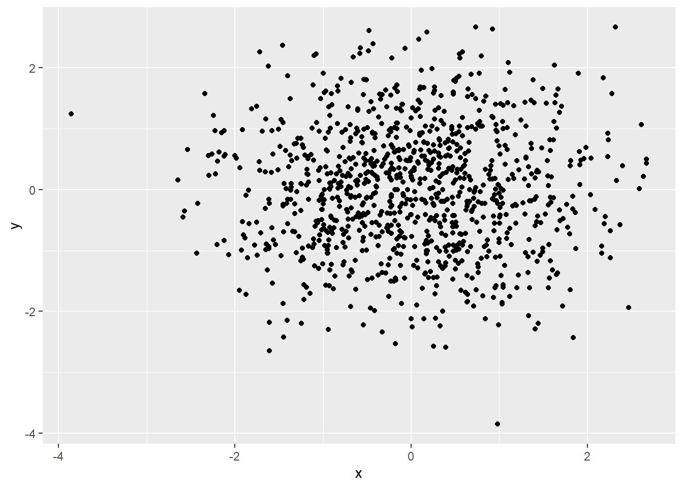
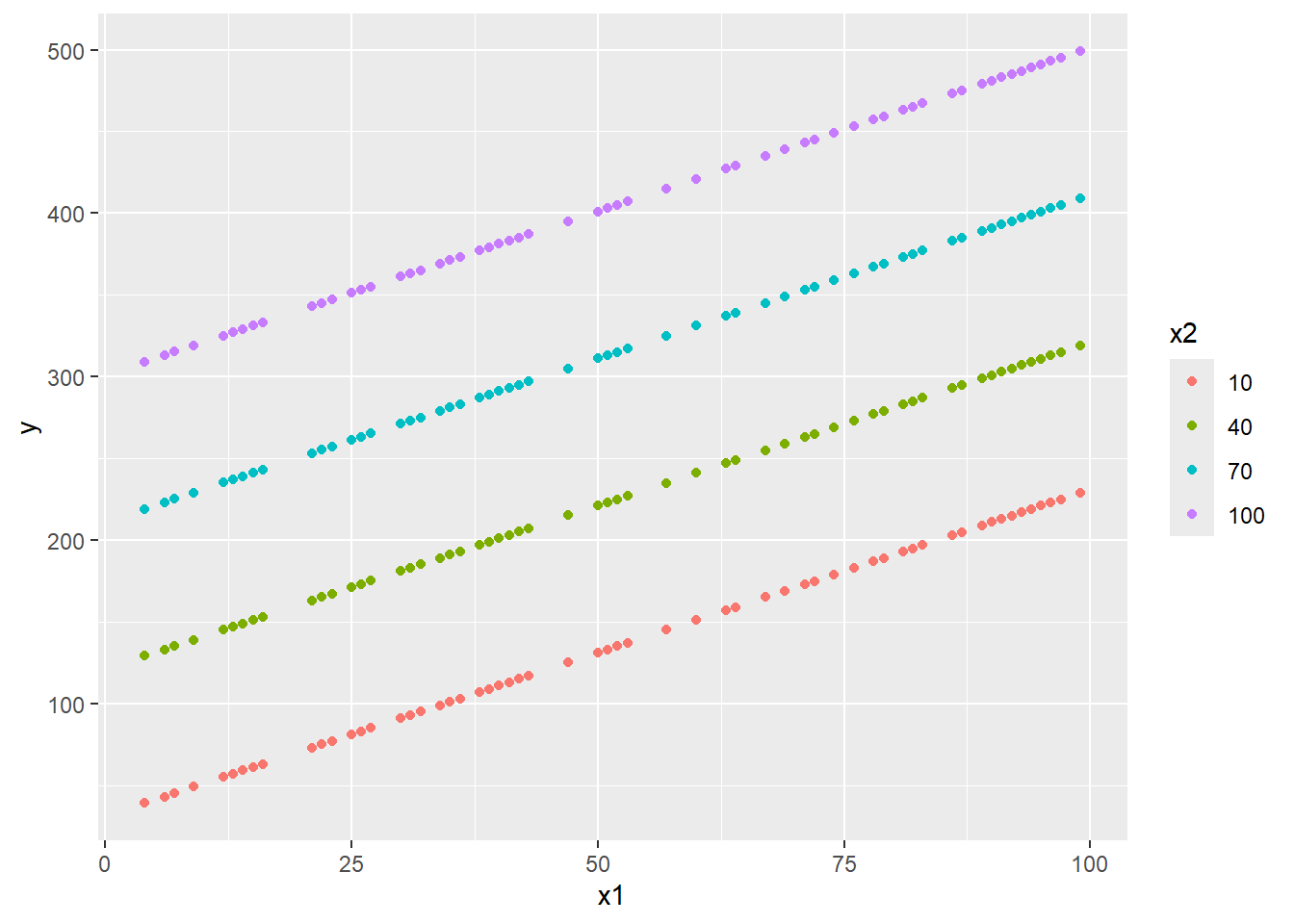
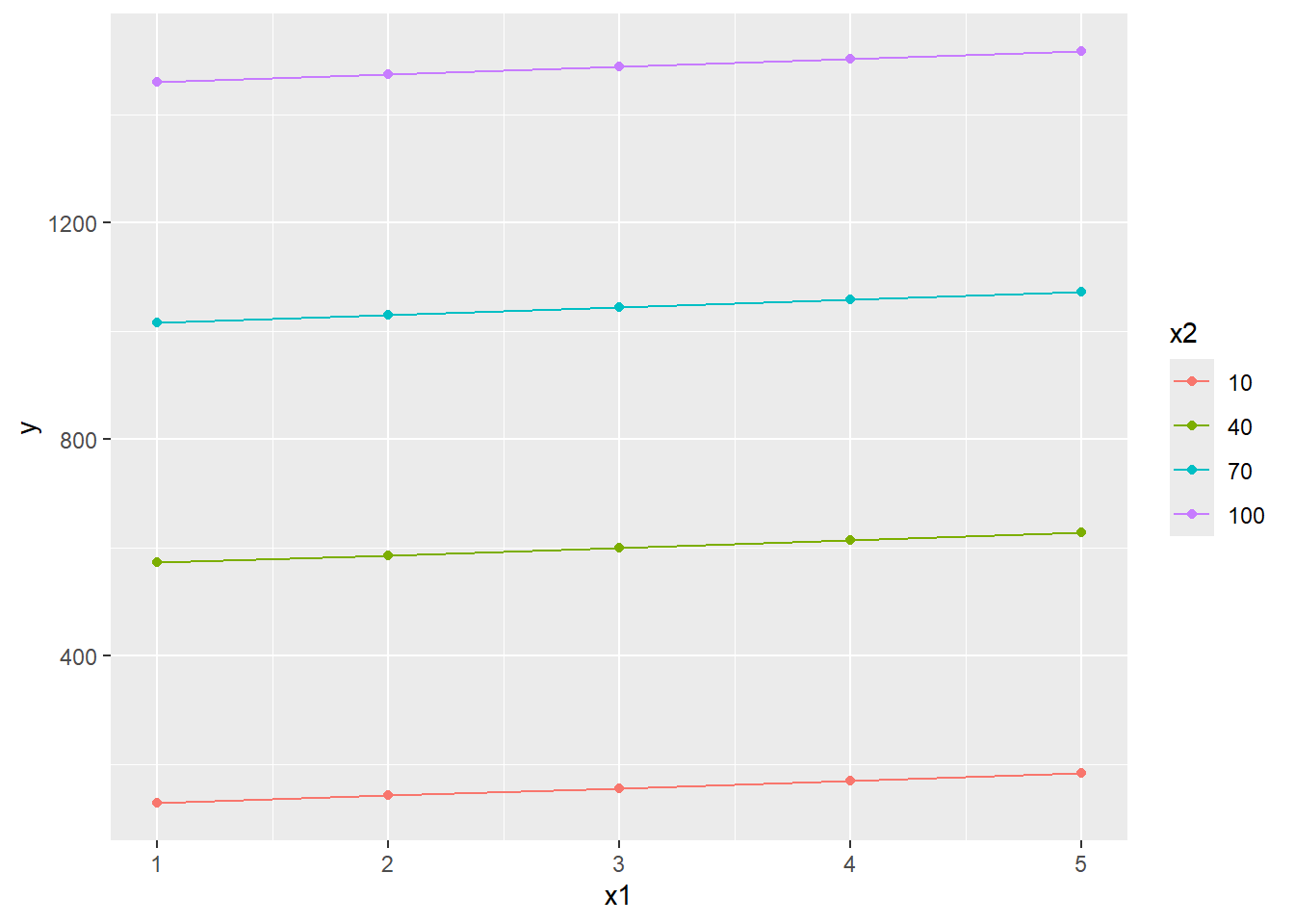
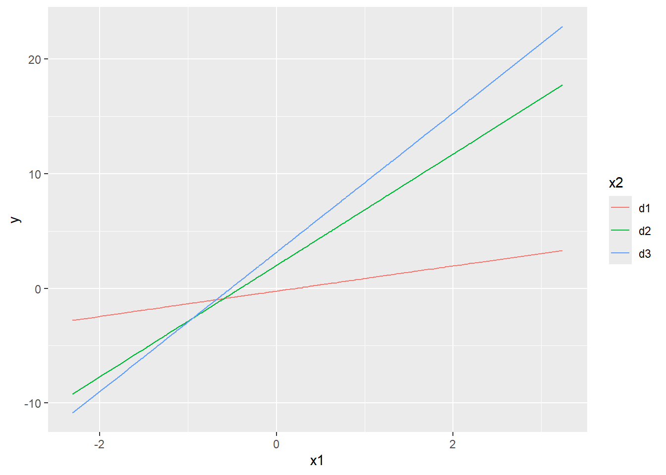
In multiple regression \[y_i=\beta_0+\beta_1x_{1i}+\cdots+\beta_px_{pi}+\epsilon_i,\] \(\beta_j\) is essentially the simple effect of \(x_j\). Multiple regression in this form is incapable of modeling interaction effect between any two independent variables. In the following visualization, it is easy to see that all lines are (destined to be) parallel to each other, implying that the model above is devoid of interaction effect.

Coding session

Assume \(\beta_0=1\), \(\beta_1=2\), \(\beta_2=3\), \(n=100\), \(\epsilon_i\in N(0,1)\).
Simulate all \(y\)s given \(y_i=\beta_0+\beta_1x_{1i}+\beta_2x_{2i}+\epsilon{i}\).
Conduct multiple regression using Mplus.

For non-quat students, do steps 3.

Simulation: multiple regression without product term can not model interaction effect

#> (Intercept)          x1          x2 
#>    0.888389    1.999498    3.001783

To incorporate interaction effect into multiple regression, we need to manually construct product term to represent interaction effect. But why does product term represent interaction effect? Let’s take a multiple regression with two independent variables as an example.

1.3.1 When \(x\)s are conitnuous

\[\begin{align*} y_i&=\beta_0+\beta_1x_{1i}+\beta_2x_{2i}+\beta_3x_{1i}x_{2i}+\epsilon_i\\ y_i&=\beta_0+(\beta_1+\beta_3x_{2i})x_{1i}+\beta_2x_{2i}+\epsilon_i\\ y_i&=\beta_0+(\beta_2+\beta_3x_{1i})x_{2i}+\beta_1x_{1i}+\epsilon_i, \end{align*}\] the effect of \(x_1\) on \(y\) is now a function of \(x_2\), and vice versa, implying that when modeling the relationship between \(x_1\) and \(y\), we take the impact of \(x_2\) into consideration by adding a product term.

Coding session

Assume \(\beta_0=1\), \(\beta_1=2\), \(\beta_2=3\), \(\beta_3 = 4\), \(n=100\), \(\epsilon_i\in N(0,1)\).
Manually construct product term \(x_1x_2\).
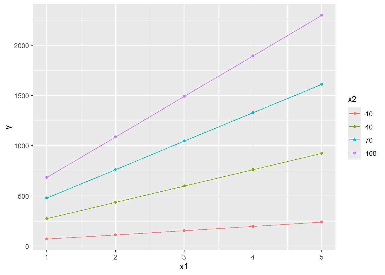
Simulate all \(y\)s given \(y_i=\beta_0+\beta_1x_{1i}+\beta_2x_{2i}+\beta_3x_{1i}x_{2i}+\epsilon{i}\).
Conduct multiple regression with and without interaction effect using Mplus.

For non-quant students, do step 4 only.

Simulation: fit multiple regression with and without product term to data that contains interaction effects

#> ------------With product term------------

#> 
#> Call:
#> lm(formula = y ~ x1 + x2 + x1x2, data = df)
#> 
#> Residuals:
#>     Min      1Q  Median      3Q     Max 
#> -3.2212 -0.6448  0.0057  0.6542  2.7976 
#> 
#> Coefficients:
#>             Estimate Std. Error t value Pr(>|t|)    
#> (Intercept)  1.46987    0.55070   2.669  0.00893 ** 
#> x1           1.99392    0.17299  11.526  < 2e-16 ***
#> x2           2.79005    0.17030  16.383  < 2e-16 ***
#> x1x2         4.01378    0.05182  77.459  < 2e-16 ***
#> ---
#> Signif. codes:  0 '***' 0.001 '**' 0.01 '*' 0.05 '.' 0.1 ' ' 1
#> 
#> Residual standard error: 1.071 on 96 degrees of freedom
#> Multiple R-squared:  0.9989, Adjusted R-squared:  0.9989 
#> F-statistic: 3.025e+04 on 3 and 96 DF,  p-value: < 2.2e-16

#> ------------Same data, without product term------------

#> 
#> Call:
#> lm(formula = y ~ x1 + x2, data = df)
#> 
#> Residuals:
#>      Min       1Q   Median       3Q      Max 
#> -17.6816  -4.8886  -0.4076   6.2894  16.4259 
#> 
#> Coefficients:
#>             Estimate Std. Error t value Pr(>|t|)    
#> (Intercept) -33.7038     2.4699  -13.65   <2e-16 ***
#> x1           14.0043     0.6081   23.03   <2e-16 ***
#> x2           14.7985     0.5588   26.48   <2e-16 ***
#> ---
#> Signif. codes:  0 '***' 0.001 '**' 0.01 '*' 0.05 '.' 0.1 ' ' 1
#> 
#> Residual standard error: 8.492 on 97 degrees of freedom
#> Multiple R-squared:  0.9329, Adjusted R-squared:  0.9315 
#> F-statistic: 674.2 on 2 and 97 DF,  p-value: < 2.2e-16

1.3.2 When \(x\)s are categrocial

1.3.2.1 No product term

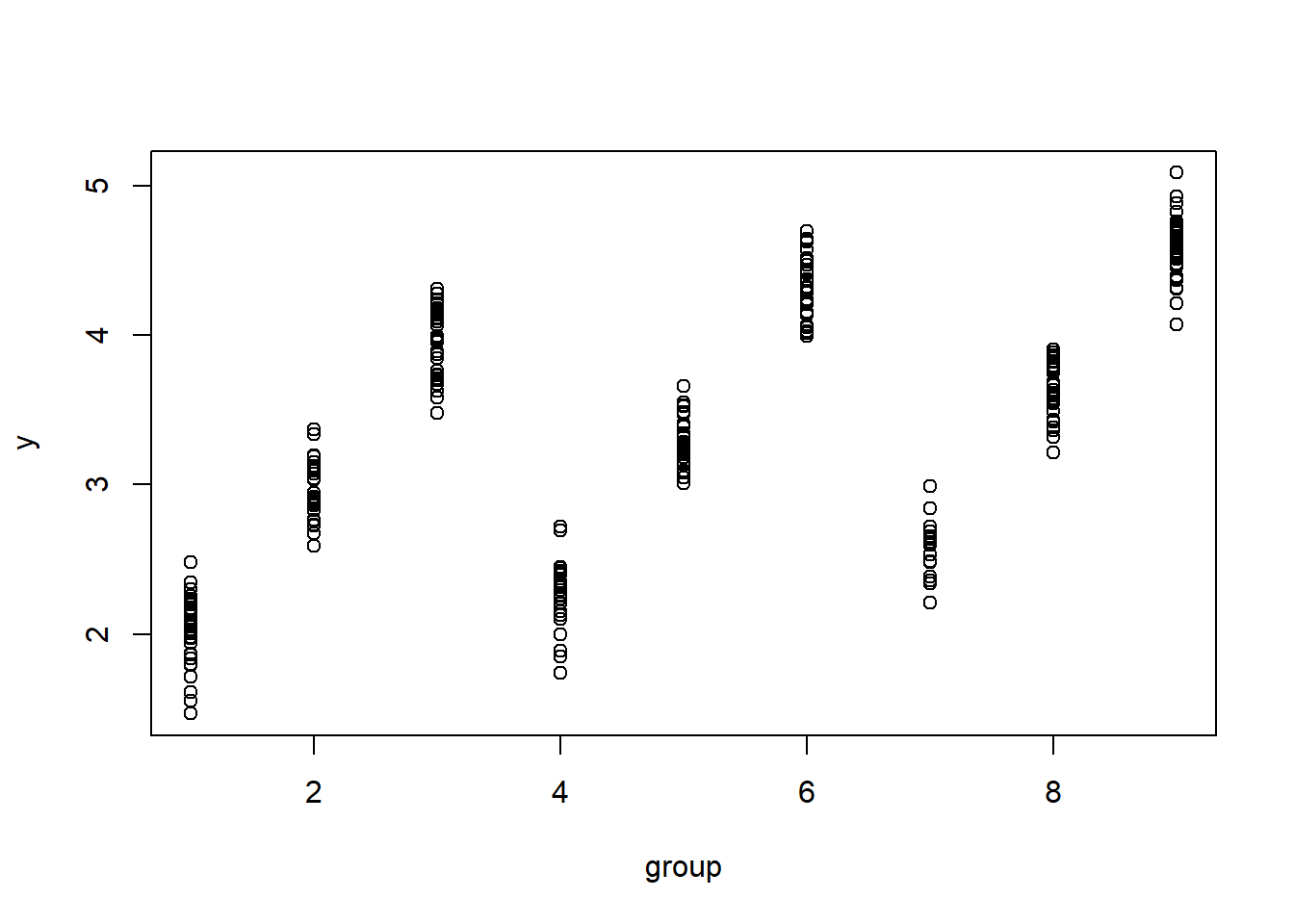
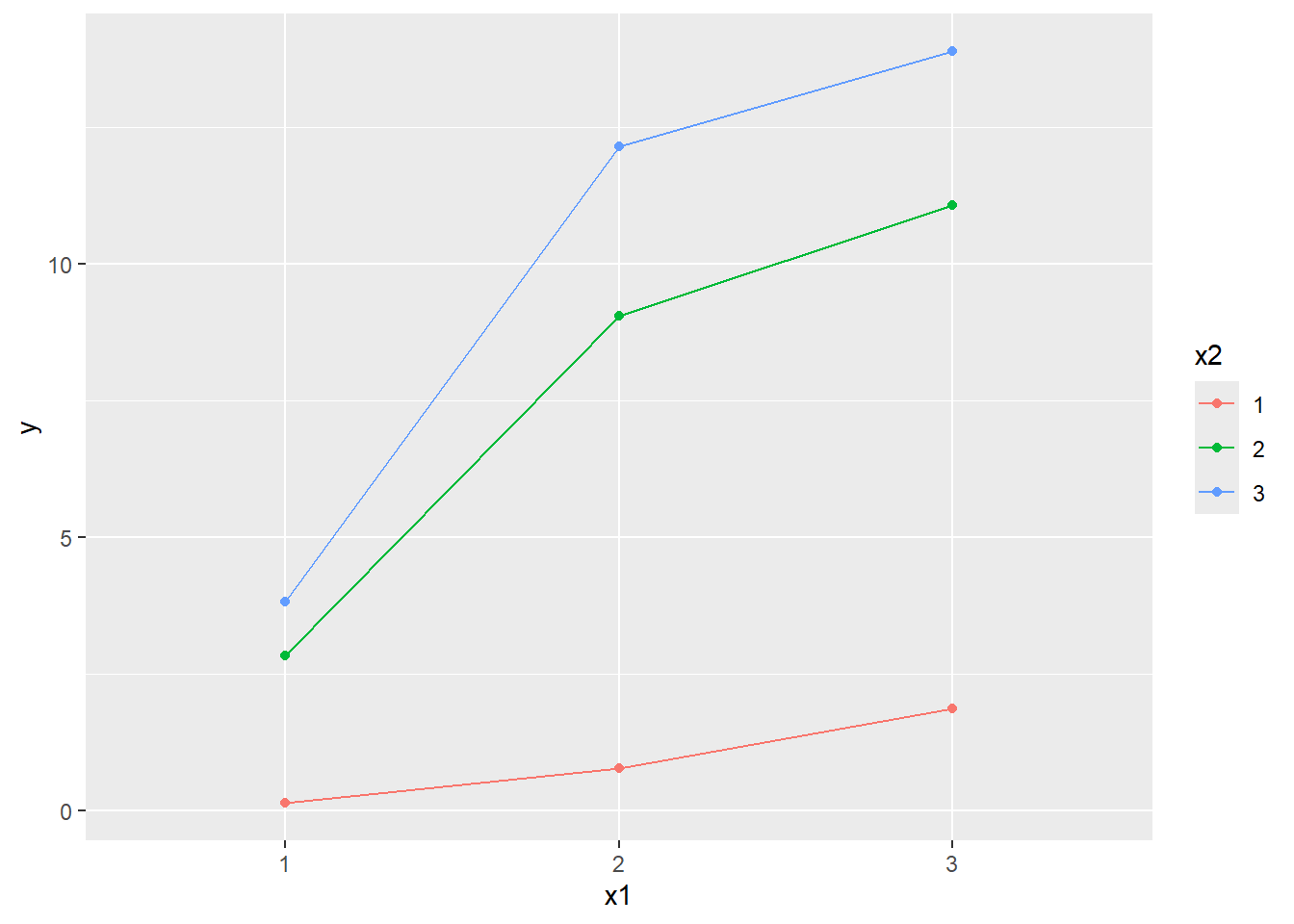
Suppose we have two categorical independent variables \(x_1\) and \(x_2\), both of which have 3 levels (1, 2, 3). We shall have two dummy variables for each \(x\) (reference categories all = 1). After dummy coding we have \[y_i=\beta_0+\beta_1d_2x_{1i}+\beta_2d_3x_{1i}+\beta_3d_2x_{2i}+\beta_4d_3x_{2i}+\epsilon_i.\]

When \(x_1=1\) and \(x_2=1\), \(d_2x_{1i}=d_3x_{1i}=d_2x_{2i}=d_3x_{2i}=0\), thus the predicted mean of this group is \[\hat{y}_{x_1=1,x_2 =1}=\hat{\beta}_0.\]

When \(x_1=2\) and \(x_2=1\), \(d_2x_{1i}=1\), \(d_3x_{1i}=d_2x_{2i}=d_3x_{2i}=0\), thus the mean of this group is \[\hat{y}_{x_1=2,x_2 =1}=\hat{\beta}_0+\hat{\beta}_1.\]

Likewise, we have the predicted mean of 9 groups as follow:

\(x_1=1,x_2=1\)	\(x_1=2,x_2=1\)	\(x_1=3,x_2=1\)
\(\hat{\beta}_0\)	\(\hat{\beta}_0+\hat{\beta}_1\)	\(\hat{\beta}_0+\hat{\beta}_2\)

\(x_1=1,x_2=2\)	\(x_1=2,x_2=2\)	\(x_1=3,x_2=2\)
\(\hat{\beta}_0+\hat{\beta}_3\)	\(\hat{\beta}_0+\hat{\beta}_1+\hat{\beta}_3\)	\(\hat{\beta}_0+\hat{\beta}_2+\hat{\beta}_3\)

\(x_1=1,x_2=3\)	\(x_1=2,x_2=3\)	\(x_1=3,x_2=3\)
\(\hat{\beta}_0+\hat{\beta}_4\)	\(\hat{\beta}_0+\hat{\beta}_1+\hat{\beta}_4\)	\(\hat{\beta}_0+\hat{\beta}_2+\hat{\beta}_4\)

Coding session

Assume \(\mu_{11}=2\), \(\mu_{21}=2.3\), \(\mu_{31}=2.6\), \(\mu_{12}=3\), \(\mu_{22}=3.3\), \(\mu_{32}=3.6\), \(\mu_{13}=4\), \(\mu_{23}=4.3\), \(\mu_{33}=4.6\), \(n=300\), \(\sigma=0.2\),
Randomly assign 300 simulated students to these 9 groups and generate their \(y\) accordingly,
Dummy code group \(x_1\) and \(x_2\), reference category = 1.
Perform multiple regression using Mplus.

For non-quant students, do steps 3-4.

#> 
#> Call:
#> lm(formula = y ~ x1 + x2, data = df)
#> 
#> Residuals:
#>      Min       1Q   Median       3Q      Max 
#> -0.56562 -0.12551  0.00952  0.13753  0.49988 
#> 
#> Coefficients:
#>             Estimate Std. Error t value Pr(>|t|)    
#> (Intercept)  1.99205    0.02418   82.38   <2e-16 ***
#> x12          0.31162    0.02741   11.37   <2e-16 ***
#> x13          0.60050    0.02837   21.17   <2e-16 ***
#> x22          1.00135    0.02885   34.71   <2e-16 ***
#> x23          1.99361    0.02875   69.35   <2e-16 ***
#> ---
#> Signif. codes:  0 '***' 0.001 '**' 0.01 '*' 0.05 '.' 0.1 ' ' 1
#> 
#> Residual standard error: 0.197 on 295 degrees of freedom
#> Multiple R-squared:  0.9525, Adjusted R-squared:  0.9518 
#> F-statistic:  1478 on 4 and 295 DF,  p-value: < 2.2e-16

Again, interaction effect is beyond the reach of a multiple regression without product term.

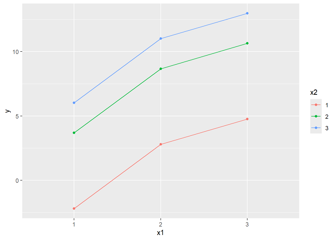
1.3.2.2 Product terms added

Now, we manually create the product terms \[\begin{align*} y_i&=\beta_0+\beta_1d_2x_{1i}+\beta_2d_3x_{1i}+\beta_3d_2x_{2i}+\beta_4d_3x_{2i}+\\ &\quad \enspace \beta_5d_2x_{1i}d_2x_{2i}+\beta_6d_2x_{1i}d_3x_{2i}+\beta_7d_3x_{1i}d_2x_{2i}+\beta_8d_3x_{1i}d_3x_{2i}+\\ &\quad \enspace \epsilon_i.\\ \end{align*}\]

Note

Note that, we need all four product terms to model the interaction effect of \(x_1\) and \(x_2\).

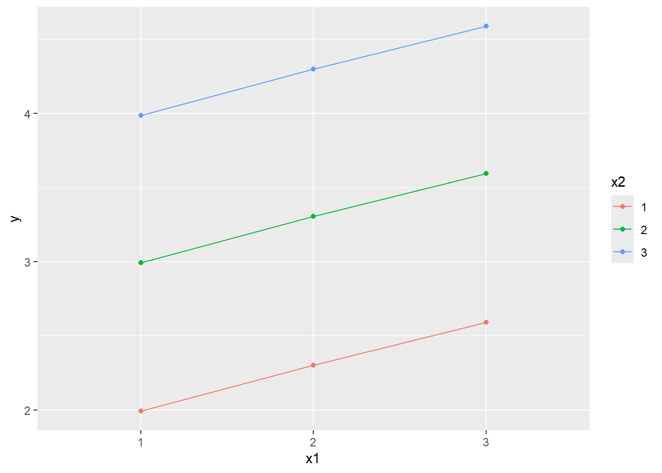
No surprise, when \(x_1=1\) and \(x_2=1\), \(d_2x_{1i}=d_3x_{1i}=d_2x_{2i}=d_3x_{2i}=0\), thus the predicted mean of this group is still the intercept \[\hat{y}_{x_1=1,x_2 =1}=\hat{\beta}_0.\]

When \(x_1=2\) and \(x_2=1\), \(d_2x_{1i}=1\), \(d_3x_{1i}=d_2x_{2i}=d_3x_{2i}=0\), thus the mean of this group is \[\hat{y}_{x_1=2,x_2 =1}=\hat{\beta}_0+\hat{\beta}_1.\]

When \(x_1=2\) and \(x_2=2\), \(d_2x_{1i}=d_2x_{2i}=1\), \(d_3x_{1i}=d_3x_{2i}=0\), thus the mean of this group is \[\hat{y}_{x_1=2,x_2 =2}=\hat{\beta}_0+\hat{\beta}_1+\hat{\beta}_3+\color{red}\hat{\beta}_5,\] where the red part represent the interaction effect between \(x_1\) and \(x_2\) when \(x_1=2\) and \(x_2=2\).

After including product terms, the predicted mean of 9 groups now become

\(x_1=1,x_2=1\)	\(x_1=2,x_2=1\)	\(x_1=3,x_2=1\)
\(\hat{\beta}_0\)	\(\hat{\beta}_0+\hat{\beta}_1\)	\(\hat{\beta}_0+\hat{\beta}_2\)

\(x_1=1,x_2=2\)	\(x_1=2,x_2=2\)	\(x_1=3,x_2=2\)
\(\hat{\beta}_0+\hat{\beta}_3\)	\(\hat{\beta}_0+\hat{\beta}_1+\hat{\beta}_3+\color{red}\hat{\beta}_5\)	\(\hat{\beta}_0+\hat{\beta}_2+\hat{\beta}_3+\color{red}\hat{\beta}_7\)

\(x_1=1,x_2=3\)	\(x_1=2,x_2=3\)	\(x_1=3,x_2=3\)
\(\hat{\beta}_0+\hat{\beta}_4\)	\(\hat{\beta}_0+\hat{\beta}_1+\hat{\beta}_4+\color{red}\hat{\beta}_6\)	\(\hat{\beta}_0+\hat{\beta}_2+\hat{\beta}_4+\color{red}\hat{\beta}_8\)

Coding session

Assume \(\beta_0 = 0\), \(\beta_1 = 1\), \(\beta_2 = 2\), \(\beta_3 = 3\), \(\beta_4 = 4\), \(\beta_5 = 5\), \(\beta_6 = 6\), \(\beta_7 = 7\), \(\beta_8 = 8\), \(n=300\), \(\epsilon_i\in N(0,1)\).
Randomly assign 300 simulated students to 9 groups.
Dummy code \(x_1\) and \(x_2\), reference category = 1.
Manually construct all product terms.
Simulate all \(y\)s according to the equation at the beginning of this subsection.
Conduct multiple regression with and without interaction effects using Mplus.

For non-quant students, do steps 3-4, and 6.

#> ------------Multiple regressio with product terms------------

#> 
#> Call:
#> lm(formula = y ~ x1d2 + x1d3 + x2d2 + x2d3 + x1d2_x2d2 + x1d3_x2d2 + 
#>     x1d2_x2d3 + x1d3_x2d3, data = df)
#> 
#> Residuals:
#>      Min       1Q   Median       3Q      Max 
#> -2.80058 -0.62138  0.04284  0.70546  2.55245 
#> 
#> Coefficients:
#>             Estimate Std. Error t value Pr(>|t|)    
#> (Intercept)   0.1397     0.1481   0.943  0.34653    
#> x1d2          0.6430     0.2402   2.677  0.00785 ** 
#> x1d3          1.7330     0.2806   6.176  2.2e-09 ***
#> x2d2          2.7028     0.2243  12.047  < 2e-16 ***
#> x2d3          3.6809     0.2243  16.407  < 2e-16 ***
#> x1d2_x2d2     5.5607     0.3371  16.493  < 2e-16 ***
#> x1d3_x2d2     6.4911     0.3660  17.737  < 2e-16 ***
#> x1d2_x2d3     7.6790     0.3360  22.854  < 2e-16 ***
#> x1d3_x2d3     8.3242     0.3650  22.808  < 2e-16 ***
#> ---
#> Signif. codes:  0 '***' 0.001 '**' 0.01 '*' 0.05 '.' 0.1 ' ' 1
#> 
#> Residual standard error: 0.9825 on 291 degrees of freedom
#> Multiple R-squared:  0.9655, Adjusted R-squared:  0.9646 
#> F-statistic:  1018 on 8 and 291 DF,  p-value: < 2.2e-16

#> ------------Dummy coding using factor------------

#> 
#> Call:
#> lm(formula = y ~ x1 + x2 + x1:x2, data = df)
#> 
#> Residuals:
#>      Min       1Q   Median       3Q      Max 
#> -2.80058 -0.62138  0.04284  0.70546  2.55245 
#> 
#> Coefficients:
#>             Estimate Std. Error t value Pr(>|t|)    
#> (Intercept)   0.1397     0.1481   0.943  0.34653    
#> x12           0.6430     0.2402   2.677  0.00785 ** 
#> x13           1.7330     0.2806   6.176  2.2e-09 ***
#> x22           2.7028     0.2243  12.047  < 2e-16 ***
#> x23           3.6809     0.2243  16.407  < 2e-16 ***
#> x12:x22       5.5607     0.3371  16.493  < 2e-16 ***
#> x13:x22       6.4911     0.3660  17.737  < 2e-16 ***
#> x12:x23       7.6790     0.3360  22.854  < 2e-16 ***
#> x13:x23       8.3242     0.3650  22.808  < 2e-16 ***
#> ---
#> Signif. codes:  0 '***' 0.001 '**' 0.01 '*' 0.05 '.' 0.1 ' ' 1
#> 
#> Residual standard error: 0.9825 on 291 degrees of freedom
#> Multiple R-squared:  0.9655, Adjusted R-squared:  0.9646 
#> F-statistic:  1018 on 8 and 291 DF,  p-value: < 2.2e-16

#> ------------Multiple regressio without product terms------------

#> 
#> Call:
#> lm(formula = y ~ x1 + x2, data = df)
#> 
#> Residuals:
#>     Min      1Q  Median      3Q     Max 
#> -4.7154 -1.2654  0.1351  1.3760  4.6007 
#> 
#> Coefficients:
#>             Estimate Std. Error t value Pr(>|t|)    
#> (Intercept)  -2.2033     0.2314  -9.523   <2e-16 ***
#> x12           4.9901     0.2623  19.026   <2e-16 ***
#> x13           6.9570     0.2714  25.633   <2e-16 ***
#> x22           5.8847     0.2760  21.322   <2e-16 ***
#> x23           8.2169     0.2751  29.874   <2e-16 ***
#> ---
#> Signif. codes:  0 '***' 0.001 '**' 0.01 '*' 0.05 '.' 0.1 ' ' 1
#> 
#> Residual standard error: 1.885 on 295 degrees of freedom
#> Multiple R-squared:  0.8713, Adjusted R-squared:  0.8696 
#> F-statistic: 499.3 on 4 and 295 DF,  p-value: < 2.2e-16

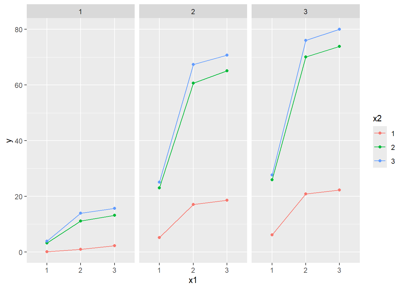
1.3.3 When having continuous \(x\) and categorical \(x\) at the same time

Assume we have one dependent variable \(y\) and two independent variables, \(x_1\) and \(x_2\), where \(x_1\) is continuous, \(x_2\) is a 3-level categorical variable. Let’s model these 3 variables with a multiple linear regression with interaction effect. First, we should dummy code \(x_2\) as \(x_2^{\text{dummy2}}\) and \(x_2^{\text{dummy3}}\) while keeping the 1st category as reference. Then we have \[\begin{align*} y_i&=\beta_0+\beta_1x_1+\beta_2x_2^{\text{dummy2}}+\beta_3x_2^{\text{dummy3}}+\beta_4x_1x_2^{\text{dummy2}}+\beta_5x_1x_2^{\text{dummy3}}+\epsilon_i.\\ \end{align*}\] When \(x_2=1\), \(x_2^{\text{dummy2}}=x_2^{\text{dummy3}}=0\), \[\begin{align*} y_i&=\beta_0+\beta_1x_1+\epsilon_i.\\ \end{align*}\] When \(x_2=2\), \(x_2^{\text{dummy2}}=1\) and \(x_2^{\text{dummy3}}=0\), \[\begin{align*} y_i&=\beta_0+\beta_1x_1+\beta_2+\beta_4x_1+\epsilon_i\\ &=(\beta_0+\beta_2)+(\beta_1+\beta_4)x_1+\epsilon_i. \end{align*}\] When \(x_2=3\), \(x_2^{\text{dummy2}}=0\) and \(x_2^{\text{dummy3}}=1\), \[\begin{align*} y_i&=\beta_0+\beta_1x_1+\beta_3+\beta_5x_1+\epsilon_i\\ &=(\beta_0+\beta_3)+(\beta_1+\beta_5)x_1+\epsilon_i, \end{align*}\] Therefore, if interaction effect between \(x_1\) and \(x_2\) was significant, we shall observe different regression relationships between \(x_1\) and \(y\) at different categories of \(x_2\).

set.seed(123)
n <- 300
x1 <- rnorm(n)
x2 <- sample(3, n, replace = TRUE)
beta_0 <- 0
beta_1 <- 1
beta_2 <- 2
beta_3 <- 3
beta_4 <- 4
beta_5 <- 5
x2d2 <- ifelse(x2 == 2, 1, 0)
x2d3 <- ifelse(x2 == 3, 1, 0)
y <- beta_0 + beta_1*x1 + beta_2*x2d2 + beta_3*x2d3 + 
  beta_4*x1*x2d2 + beta_5*x1*x2d3 + rnorm(n)
df <- data.frame(x1 = x1, x2 = x2, y = y)
df$x2 <- factor(df$x2)
fit <- lm(y ~ x1 + x2 + x1:x2, data = df)
summary(fit)

#> 
#> Call:
#> lm(formula = y ~ x1 + x2 + x1:x2, data = df)
#> 
#> Residuals:
#>     Min      1Q  Median      3Q     Max 
#> -2.6102 -0.6499  0.0805  0.6481  2.7053 
#> 
#> Coefficients:
#>             Estimate Std. Error t value Pr(>|t|)    
#> (Intercept)  -0.2435     0.1016  -2.397   0.0172 *  
#> x1            1.1009     0.1103   9.982   <2e-16 ***
#> x22           2.2499     0.1441  15.611   <2e-16 ***
#> x23           3.4034     0.1379  24.688   <2e-16 ***
#> x1:x22        3.7590     0.1494  25.167   <2e-16 ***
#> x1:x23        4.9766     0.1511  32.926   <2e-16 ***
#> ---
#> Signif. codes:  0 '***' 0.001 '**' 0.01 '*' 0.05 '.' 0.1 ' ' 1
#> 
#> Residual standard error: 0.9816 on 294 degrees of freedom
#> Multiple R-squared:  0.9577, Adjusted R-squared:  0.957 
#> F-statistic:  1332 on 5 and 294 DF,  p-value: < 2.2e-16

coefs <- coef(fit)
data.frame(
  x1 = x1, 
  y_d1 = coefs[1] + coefs["x1"]*x1,
  y_d2 = (coefs[1] + coefs["x22"]) + (coefs["x1"] + coefs["x1:x22"])*x1,
  y_d3 = (coefs[1] + coefs["x23"]) + (coefs["x1"] + coefs["x1:x23"])*x1, 
  row.names = NULL
) |> 
  pivot_longer(
    cols = 2:4, 
    names_sep = "_", 
    names_to = c(NA, "x2"), 
    values_to = "y"
  ) |>
ggplot(aes(x = x1, y = y, color = x2)) + 
  geom_line()

1.4 Tricks

1.4.1 Re-organize GLM’s results into an ANOVA style

Reference: Why do the anova() and summary() functions produce different significance values for linear models?

1.4.2 Remove unwanted interaction effect

When doing empirical research, it is not unusual to have more than 3 categorical \(x\)s. The resulting regression model quickly becomes cumbersome to deal with because of many interaction effects involved. In SPSS, the default of ANOVA is including all possible interaction effects. In ANOVA, each hypothesis corresponds to an effect (main, interaction, simple), the default setting of SPSS easily leads to redundant hypotheses when having multiple categorical \(x\)s. However, given the confirmatory nature (testing hypothesis) of empirical research in psychology, the number of focal hypotheses is usually limited in a single study. To reduce the number of hypotheses, a common practice is removing all interaction effects that are not of interest. Following is an example of a 3-way design with a specific second order interaction effect removed.

# Straight forward solution in R
set.seed(123)
n <- 900
df <- data.frame(
  program = sample(1:3, size = n, replace = TRUE),
  school = sample(1:3, size = n, replace = TRUE),
  division = sample(1:3, size = n, replace = TRUE),
  height = sample(3:7, size = n, replace = TRUE)
)
df$program <- factor(df$program)
df$school <- factor(df$school)
df$division <- factor(df$division)
# Default: model all interaction effects at once
fit_all <- lm(
  height ~ program + school + division + program*school*division, 
  data = df
)
summary(fit_all)

#> 
#> Call:
#> lm(formula = height ~ program + school + division + program * 
#>     school * division, data = df)
#> 
#> Residuals:
#>     Min      1Q  Median      3Q     Max 
#> -2.6585 -1.0000  0.0625  1.1071  2.5769 
#> 
#> Coefficients:
#>                            Estimate Std. Error t value Pr(>|t|)    
#> (Intercept)                 5.05882    0.23473  21.551  < 2e-16 ***
#> program2                   -0.37132    0.33711  -1.101  0.27098    
#> program3                   -0.05882    0.33711  -0.174  0.86152    
#> school2                    -0.42246    0.31253  -1.352  0.17681    
#> school3                    -0.63575    0.35658  -1.783  0.07495 .  
#> division2                  -0.16597    0.34929  -0.475  0.63480    
#> division3                  -0.12132    0.33711  -0.360  0.71901    
#> program2:school2            0.49358    0.46991   1.050  0.29384    
#> program3:school2            0.07871    0.46342   0.170  0.86517    
#> program2:school3            1.44825    0.49814   2.907  0.00374 ** 
#> program3:school3            0.58813    0.47990   1.226  0.22070    
#> program2:division2          0.40154    0.50259   0.799  0.42454    
#> program3:division2          0.08702    0.47942   0.182  0.85601    
#> program2:division3          0.33859    0.46561   0.727  0.46730    
#> program3:division3         -0.20300    0.47203  -0.430  0.66726    
#> school2:division2           0.41849    0.48370   0.865  0.38717    
#> school3:division2           1.06432    0.51085   2.083  0.03750 *  
#> school2:division3           0.21223    0.46151   0.460  0.64572    
#> school3:division3           0.40877    0.48476   0.843  0.39932    
#> program2:school2:division2  0.24585    0.68910   0.357  0.72135    
#> program3:school2:division2  0.32563    0.68356   0.476  0.63392    
#> program2:school3:division2 -2.01418    0.72174  -2.791  0.00537 ** 
#> program3:school3:division2 -1.34952    0.68448  -1.972  0.04897 *  
#> program2:school2:division3 -0.01669    0.65898  -0.025  0.97980    
#> program3:school2:division3  0.32541    0.67982   0.479  0.63230    
#> program2:school3:division3 -1.01492    0.67277  -1.509  0.13177    
#> program3:school3:division3  0.02984    0.65605   0.045  0.96374    
#> ---
#> Signif. codes:  0 '***' 0.001 '**' 0.01 '*' 0.05 '.' 0.1 ' ' 1
#> 
#> Residual standard error: 1.369 on 873 degrees of freedom
#> Multiple R-squared:  0.0415, Adjusted R-squared:  0.01295 
#> F-statistic: 1.454 on 26 and 873 DF,  p-value: 0.06725

anova(fit_all)

# remove unwanted interaction effect by using the update() function
#   e.g. remove the interaction effect of program and division
fit_part <- update(fit_all, ~.-program:division)
summary(fit_part)

#> 
#> Call:
#> lm(formula = height ~ program + school + division + program:school + 
#>     school:division + program:school:division, data = df)
#> 
#> Residuals:
#>     Min      1Q  Median      3Q     Max 
#> -2.6585 -1.0000  0.0625  1.1071  2.5769 
#> 
#> Coefficients:
#>                            Estimate Std. Error t value Pr(>|t|)    
#> (Intercept)                 5.05882    0.23473  21.551  < 2e-16 ***
#> program2                   -0.37132    0.33711  -1.101  0.27098    
#> program3                   -0.05882    0.33711  -0.174  0.86152    
#> school2                    -0.42246    0.31253  -1.352  0.17681    
#> school3                    -0.63575    0.35658  -1.783  0.07495 .  
#> division2                  -0.16597    0.34929  -0.475  0.63480    
#> division3                  -0.12132    0.33711  -0.360  0.71901    
#> program2:school2            0.49358    0.46991   1.050  0.29384    
#> program3:school2            0.07871    0.46342   0.170  0.86517    
#> program2:school3            1.44825    0.49814   2.907  0.00374 ** 
#> program3:school3            0.58813    0.47990   1.226  0.22070    
#> school2:division2           0.41849    0.48370   0.865  0.38717    
#> school3:division2           1.06432    0.51085   2.083  0.03750 *  
#> school2:division3           0.21223    0.46151   0.460  0.64572    
#> school3:division3           0.40877    0.48476   0.843  0.39932    
#> program2:school1:division2  0.40154    0.50259   0.799  0.42454    
#> program3:school1:division2  0.08702    0.47942   0.182  0.85601    
#> program2:school2:division2  0.64739    0.47144   1.373  0.17003    
#> program3:school2:division2  0.41265    0.48725   0.847  0.39728    
#> program2:school3:division2 -1.61264    0.51799  -3.113  0.00191 ** 
#> program3:school3:division2 -1.26250    0.48853  -2.584  0.00992 ** 
#> program2:school1:division3  0.33859    0.46561   0.727  0.46730    
#> program3:school1:division3 -0.20300    0.47203  -0.430  0.66726    
#> program2:school2:division3  0.32190    0.46634   0.690  0.49021    
#> program3:school2:division3  0.12241    0.48922   0.250  0.80249    
#> program2:school3:division3 -0.67634    0.48563  -1.393  0.16406    
#> program3:school3:division3 -0.17316    0.45562  -0.380  0.70399    
#> ---
#> Signif. codes:  0 '***' 0.001 '**' 0.01 '*' 0.05 '.' 0.1 ' ' 1
#> 
#> Residual standard error: 1.369 on 873 degrees of freedom
#> Multiple R-squared:  0.0415, Adjusted R-squared:  0.01295 
#> F-statistic: 1.454 on 26 and 873 DF,  p-value: 0.06725

anova(fit_part)

# Workaround solution for Mplus user
# Step 1: create the design matrix with all terms included
term_all <- model.matrix(
  height ~ program + school + division + program*school*division, 
  data = df
)
head(term_all)
# Step 2: remove all terms associated with unwanted interaction effects
id_column_omit <- grep("program[2-3][:]division[2-3]", colnames(term_all))
xs <- term_all[, -id_column_omit]
# Mplus model intercept in default, we need to remove the intercept 
#   column from design matrix to avoid having redundant intercept

# Step 3: combine the model matrix with dependent variable
df_part <- cbind(xs[, -1], df$height)
head(df_part)
# Step 4: save the data as local file
write.table(
  df_part,
  file = paste(
    getwd(),
    "/data/1y 3xs_categorical_interaction_remove_unwanted_interaction.txt",
    sep = ""
  ),
  col.names = FALSE,
  row.names = FALSE
)

Reference: