3 When \(y\) is categorical: generalized linear model
3.1 Categorical dependent variable
Normal regression requires the dependent variable (DV) \(y\) to be continuous. However, \(y\) can be categorical. To accurately model categorical \(y\), we need new regression model.
3.2 Basic logic of modeling categorical \(y\)
In normal regression, we have
\[y_i=\beta_0+\beta_1x_{1i}+\cdots+\beta_px_{pi}+\epsilon_i,\]
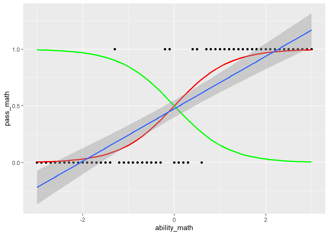
where \(\epsilon_i\in N(0,\sigma^2)\). Since \(\epsilon_i\) is continuous, \(y_i\) must be continuous. If we model categorical DV using normal regression, treating categorical \(y\) as continuous, it will definitely lead to a very poor model fit.
No matter what the nature of DV is (discrete or continuous), we are interested in the linear relationship between \(y\) and background variables \(\boldsymbol{x}\). This means that the regression model for discrete \(y\) has a right hand side (\(\beta_0+\beta_1x_{1i}+\cdots+\beta_px_{pi}\)) similar to that of the regression model for continuous \(y\), they only differ in the left hand side.
Because multiple regression requires its left hand side to be continuous, we have to transform (one-one mapping, i.e. monotonic transformation) categorical \(y\) into continuous one, \(y^*\), and put \(y^*\) in the left hand side instead. This contains two steps:
- model probability: treat categorical \(y\) as observations of an discrete random variable with probability mass function, and modeling their probabilities instead;
- convert probability: convert probability \((0,1)\) into fully continuous scale \((-\infty,+\infty)\) using link function.
3.2.1 Probability behind categorical \(y\)
We treat categorical \(y\) as observations of a discrete random variable \(Y\) with \(K\) particular values, it follows
\[\begin{cases}P(Y=y_1)\\P(Y=y_2)\\\cdots\\P(Y=y_K)\\\end{cases}.\]
Now we only need to transform ranged continuous \(P\)s into unranged continuous \(y^*\), this is realized through link function.
3.2.2 Link function
The general form of link function is \(f(y)=y^*\), the resultant regression model is \[f[P(Y=y_k)]=y^*=\beta_{0k}+\beta_{1k}x_1+\cdots+\beta_{pk}x_p.\]
The subscript \(k\) implies that there will be \(K-1\) regression models, because we have \(K\) \(P\)s and their summation must be 1. If \(y\) is dichotomous (1 or 0), \[\begin{align*}
f[P(Y=1)]=y^*&=\beta_0+\beta_1x_1+\cdots+\beta_px_p\\
P(Y=1)&=f^{-1}(\beta_0+\beta_1x_1+\cdots+\beta_px_p),
\end{align*}\] then \[P(Y=0) = 1 - f^{-1}(\beta_0+\beta_1x_1+\cdots+\beta_px_p).\] That is, we only need 1 regression model for dichotomous \(y\).
If these \(K-1\) models fit the data well, the predicted probabilities will match the observed \(y\) closely as a whole. \(K-1\) regression models can be computationally complex in high dimension, especially for the nominal probit regression.
Unlike multiple regression, there is no error term in the resultant regression model for categorical \(y\). This is echoed in many text,
- Why do we model noise in linear regression but not logistic regression?
- Logistic Regression - Error Term and its Distribution
- Estimating the error term in a logistic regression
- Error distribution for linear and logistic regression
to name a few. Readers interested in a more detailed explanation are refereed to Hosmer et al. (2013), page 7.
However, there also exists a statement that regression models for categorical \(y\) contain error terms, the resultant regression models have latent variables and are called threshold models. Mplus uses this latent variable framework (Muthén, 1998-2004).
- Probit model
- Probit classification model, or probit regression
- Relationship between the latent variable as a function of regressors and the logit model?
- Estimating the error term in a logistic regression
- The Latent Variable Model in Binary Regressions
Actually, these two seemingly conflicting statements unite, regression models without error terms and threshold models are equivalent (see Section 3.4.1.1 for more detail). But for consistency, we still use the ones with no error term through this chapter.
3.3 Why distinguishing between nominal and ordinal?
TODO: Need an example, could be simulation or mathematical derivation
Categorical \(y\) can be either nominal or ordinal. Ordinal variable contains information about trend. By using this ordinal nature of the variable, we can narrow down the scope of alternative hypotheses and increase the power of statistical tests. Models with terms that reflect ordinal characteristics such as monotone trend have improved model parsimony and power. That is why people tend to treat nominal as ordinal.
3.4 When \(y\) is nominal
3.4.1 Nominal probit regression
Because we need a link function that can transform \(P(Y=y) \in(0,1)\) into \(y^*\in(-\infty, +\infty)\), and vice versa. Actually, there exists a well-known function that meet this requirement, i.e. the cumulative distribution function of standard normal distribution:
\[\phi(z)=\int^{z}_{-\infty}f(z)dx=P(Z<=z),\]
where \(z\in N(\mu,\sigma^2)\), lies in \((-\infty, +\infty)\), \(f(z)\) is the probability density function, and \(\phi(z)\in(0,1)\). Thus,
\[\begin{align*} z&=\phi^{-1}[P(Z<=z)] \end{align*}\] Now we only need to convert \(P(Y=y_k)\) into \(\phi(z_k)=P(Z_k<=z_k)\).
3.4.1.1 Threshold \(\tau\): the nominal probit regression as a latent variable model
The following text is mainly based on the chapter 7.1.1 of Agresti’s book (2013).
To model categorical \(y\), we first target probability \(P(Y=y_k)\) instead of observed \(y\). We then convert \(P(Y=y_k)\) into fully continuous \(y^*\) using link function. This is equivalent to a latent variable model assuming that there is an unobserved continuous random variable \(y^*\), such that the observed response \(y\neq y_k\) if \(y^*\leq\tau_k\) and \(y=y_k\) if \(y>\tau_k\), \[\begin{align*} P(Y=y_k)=P(y^*>\tau_k)&=P(\beta_{0k}+\beta_{1k}x_1+\cdots+\beta_{pk}x_p+\epsilon_{k}>\tau_k), \end{align*}\] where \(\epsilon_{k}\) are independent from \(N(0,\sigma^2)\). \[\begin{align*} P(y^*>\tau_k)&=P(-\epsilon_{k}<\beta_{0k}+\beta_{1k}x_1+\cdots+\beta_{pk}x_p-\tau_k)\\ &=P\left(-Z_{\epsilon_k}<\frac{\beta_{0k}+\beta_{1k}x_1+\cdots+\beta_{pk}x_p-\tau_k}{\sigma}\right), \end{align*}\] where \(-\epsilon_k\) has the same distribution as \(\epsilon_k \in N(0,\sigma^2)\), so do \(-Z_{\epsilon_k}\) and \(Z_{\epsilon_k} \in N(0,1)\). Now we successfully convert \(P(Y=y_k)\) into \(\phi(z_k)=P(Z_k<=z_k)\), where \(\phi\) is cumulative density function of standard normal distribution, \(Z_k=-Z_{\epsilon_k}\), and \(z_k=(\beta_{0k}+\beta_{1k}x_1+\cdots+\beta_{pk}x_p-\tau)/(\sigma_{\epsilon_{k}})\). To make this model identifiable, it is common to arbitrarily set \(\sigma=1\) and \(\tau_k=0\), resulting \[\begin{align*} P(y^*>0)&=P(-Z_{\epsilon_k}<\beta_{0k}+\beta_{1k}x_1+\ldots+\beta_{pk}x_p)\\ &=\phi(\beta_{0k}+\beta_{1k}x_1+\cdots+\beta_{pk}x_p), \end{align*}\] this is why we do not need to estimate \(\sigma\) for probit regression as the case in normal regression. Stats tool with such setting (i.e. the glm function in R) will report estimated intercepts, but no estimated thresholds.
Some statistical software does not include intercept in the right hand side, therefore \[\begin{align*} P(y^*>\tau_k)&=P(\beta_{1k}x_1+\cdots+\beta_{pk}x_p+\epsilon_{k}>\tau_k)\\ &=P(-\epsilon_{k}<-\tau_k+\beta_{1k}x_1+\cdots+\beta_{pk}x_p)\\ &=P\left(-Z_{\epsilon_k}<\frac{-\tau_k+\beta_{1k}x_1+\cdots+\beta_{pk}x_p}{\sigma}\right)\\ &=\phi(-\tau_k+\beta_{1k}x_1+\cdots+\beta_{pk}x_p), \end{align*}\] then \(-\tau_k\) becomes the intercepts, we only need to set \(\sigma=1\) to make this model identifiable. Stats tool with such setting (i.e. Mplus) will report estimated thresholds, but no estimated intercepts.
3.4.2 Baseline-category logistic regression
Logistic regression uses another link function, log odd.
For a discrete random variable \(Y\) with \(K\) values, the odd of \(y_1\) is defined as
\[Odd[P(Y=y_{1})]=\frac{P(Y=y_1)}{P(Y=y_K)},\]
where \(P(Y=y_K)\) is reference probability of baseline-category. We usually use the last category or the most common one as the baseline. This is an arbitrary choice.
Odd use the reference probability as unit to measure \(P(Y=y_1)\). It is easy to see that \(Odd\in(0,+\infty)\), therefore we convert probability \((0,1)\) into \((0,+\infty)\), the last step is further convert Odd into \((-\infty,+\infty)\). Natural logarithm perfectly fulfill the need. The resulting logistic regression is \[\begin{align*} \log\left[\frac{P(Y=y_1)}{P(Y=y_K)}\right]&=\beta_{01}+\beta_{11}x_1+\cdots+\beta_{p1}x_p\\ P(Y=y_1)&=P(Y=y_K)\exp(\beta_{01}+\beta_{11}x_1+\cdots+\beta_{p1}x_p)\\ &=P(Y=y_K)\exp([1,\boldsymbol{x}']\boldsymbol{\beta}_1). \end{align*}\] It is easy to see that \[\begin{align*} P(Y=y_2)&=P(Y=y_K)\exp([1,\boldsymbol{x}']\boldsymbol{\beta}_2)\\ &\quad\cdots\\ P(Y=y_{K-1})&=P(Y=y_K)\exp([1,\boldsymbol{x}']\boldsymbol{\beta}_{K-1}). \end{align*}\] Because \(\sum_{k-1}^{K}P(Y=y_k)=1\), we have \[\begin{align*} P(Y=y_K)[\exp([1,\boldsymbol{x}']\boldsymbol{\beta}_1)+\cdots+\exp([1,\boldsymbol{x}']\boldsymbol{\beta}_{K-1})]+P(Y=y_K)=1, \end{align*}\] thus \[\begin{align*} P(Y=y_K)&=\frac{1}{1+\exp([1,\boldsymbol{x}']\boldsymbol{\beta}_1)+\cdots+\exp([1,\boldsymbol{x}']\boldsymbol{\beta}_{K-1})}. \end{align*}\]
For dichotomous \(y\), \[Odd[P(Y=1)]=\frac{P(Y=1)}{1- P(Y=1)}.\]
The regression model is \[\begin{align*} \log\left[\frac{P(Y=1)}{1-P(Y=1)}\right]&=\beta_0+\beta_1x_1+\cdots+\beta_px_p\\ \frac{P(Y=1)}{1-P(Y=1)}&=\exp(\beta_0+\beta_1x_1+\cdots+\beta_px_p)\\ P(Y=1)&=[1-P(Y=1)]\exp(\beta_0+\beta_1x_1+\cdots+\beta_px_p)\\ P(Y=1)&=\frac{\exp(\beta_0+\beta_1x_1+\cdots+\beta_px_p)}{1+\exp(\beta_0+\beta_1x_1+\cdots+\beta_px_p)}\\ &=\frac{1}{1+\exp(-\beta_0-\beta_1x_1-\cdots-\beta_px_p)}. \end{align*}\]
Both the logistic regression and probit regression can be estimated through maximum likelihood, the detail is omitted here.
3.4.2.1 Threshold \(\tau_k\): the norminal logistic regression as a latent variable model
Similar to probit regression, baseline logistic regression can also be viewed as a latent variable model. The only difference is that \(\epsilon_{k}\) are now independently from standardize logistic distribution \[\begin{align*} P(Y=y_k)=P(y^*>\tau_k)&=P(\beta_{0k}+\beta_{1k}x_1+\cdots+\beta_{pk}x_p+\epsilon_{k}>\tau_k)\\ &=P(\frac{-\epsilon_{k}}{\sigma}<\frac{-\tau_k+\beta_{0k}+\beta_{1k}x_1+\cdots+\beta_{pk}x_p}{\sigma})\\ &=G(\beta_{0k}+\beta_{1k}x_1+\cdots+\beta_{pk}x_p-\tau_k), \end{align*}\] where \(\tau_k=0\) for identifiability, \(G\) is the cumulative density function of standardize logistic distribution. Although a standard logistic distribution has \(\mu=0\) and \(\sigma^2=\pi^2/3\),\(\sigma^2\) only will affect the scaling of parameters but not the predicted probabilities, we could simply set \(\sigma^2=1\).
3.4.2.2 Odd ratio
Odds ratio in logistic regression can be interpreted as the effect of one unit of change in \(x_j\) in the predicted odds ratio while holding other background variables at constant, \[OR[P(Y=y_1)|_{x_j}]=\frac{Odd[P(Y=y_1|x_j+1)]}{Odd[P(Y=y_1|x_j)]}.\] Because \[\begin{align*} Odd[P(Y=y_1)]&= \frac{P(Y=y_1)}{P(Y=y_k)}\\ &= \frac{P(Y=y_k)\exp(\beta_{01}+\beta_{11}x_1+\cdots+\beta_{p1}x_p)}{P(Y=y_k)}\\ &=\exp(\beta_{01}+\beta_{11}x_1+\cdots+\beta_{p1}x_p), \end{align*}\] then \[\begin{align*} OR[P(Y=y_1)|_{x_j}]&=\frac{\exp[\beta_{01}+\beta_{11}x_1+\ldots+\beta_{j1}(x_j+1)+\ldots+\beta_{p1}x_p]}{\exp(\beta_{01}+\beta_{11}x_1+\ldots+\beta_{j1}x_j+\ldots+\beta_{p1}x_p)}\\ &=\exp(\beta_{j1}). \end{align*}\]
3.4.2.3 Visualization of probabilities: nominal logistic regression
Following is the visualization of the nominal logistic regression model of ex.3.6.
3.5 When \(y\) is ordinal
3.5.1 Culmulative probability
Because the categories of \(y\) now have order, for a K-level ordinal \(y\), \[\begin{align*} \begin{cases} y=1,\text{ if }y^*\leq\tau_1\\ y=2,\text{ if }\tau_1< y^*\leq\tau_2\\ \cdots\\ y=K,\text{ if }\tau_{K-1}<y^*. \end{cases} \end{align*}\] The cumulative probability is \[P(Y\le y_j)=P(Y=y_1)+\cdots+P(Y=y_j).\]
3.5.2 Cumulative probit regression
In nominal case, \(P(Y=y_k)\) is treated as cumulative probability of a standard normal random variable \(Z_k\). The modeled probability is now cumulative already, we are effectively treating \(P(Y\leq y_1),P(Y\leq y_2),\cdots,P(Y\leq y_k)\) as cumulative probabilities of a common random variable \(Z\), therefore we have a more parsimonious model:
\[\phi^{-1}[P(Y\leq y_k)]=y^*=\beta_{0k}+\beta_1x_1+\cdots+\beta_px_p.\]
3.5.2.1 Threshold \(\tau_k\): the ordinal probit regression as a latent variable model
When \(y\) is ordinal, we then model \(P(Y\leq y_j)\) as the cumulative probability of a latent variable \(y^*\) with \(\tau_k\) as \[\begin{align*} \phi^{-1}[P(Y\leq y_k)]&=\phi^{-1}[P(y^*<\tau_k)] \\ P(y^*<\tau_k)&=\beta_{0k}+\beta_1x_1+\cdots+\beta_px_p+\epsilon_k<\tau_k, \end{align*}\] where \(\epsilon_k\in N(0,\sigma^2)\), \[\begin{align*} P(y^*<\tau_k)&=P(\epsilon_k<\tau_k-\beta_{0k}-\beta_1x_1-\cdots-\beta_px_p)\\ &=P(\frac{\epsilon_k}{\sigma}<\frac{\tau_k-\beta_{0k}-\beta_1x_1-\cdots-\beta_px_p}{\sigma}). \end{align*}\] To make this model identifiable, let \(\sigma=1\) and \(\tau_k=0\), then \[\begin{align*} P(y^*<\tau_k)=P(Z_{\epsilon_k}<-\beta_{0k}-\beta_1x_1-\cdots-\beta_px_p). \end{align*}\] It is easy to see that, the signs of all regression coefficients of ordinal probit regression are negative.
In statistical software (i.e. Mplus) modeling ordinal probit model without an intercept, \(\tau_k\) replaces the intercept \[\begin{align*} P(y^*<\tau_k)=P(Z_{\epsilon_k}<\tau_k-\beta_1x_1-\cdots-\beta_px_p). \end{align*}\]
\(\tau_k\) in ordinal logistic regression is similar to that in ordinal probit regression, thus is omitted.
3.5.3 Cumulative logistic regression
The odd of cumulative logistic regression becomes
\[Odd[P(Y\leq y_k)]=\frac{P(Y\leq y_k)}{1 - P(Y\leq y_K)}.\]
A model for \(\log odd(P(Y\leq y_k))\) alone is an ordinary logistic model for a binary response in which categories 1 to \(k\) form one outcome and categories \(k+1\) to \(K\) form the second. The model that simultaneously uses all \(K-1\) cumulative log odds in a single parsimonious model is \[\begin{align*} \log\left[\frac{P(Y\leq y_k)}{1 - P(Y\leq y_k)}\right]&=\beta_{0k}+\beta_1x_1+\cdots+\beta_px_p.\\ \end{align*}\] Each cumulative logit has its own intercept. The \(\beta_{0k}\) are increasing in \(k\), because \(P(Y\leq y_k)\) increases in \(k\) for fixed \(\boldsymbol{x}\) and the logit is an increasing function of \(P(Y\leq y_k)\). This model assumes slopes remian the same for each logit. This is also called parallel slopes assumption and can be seen clearly in Section 3.5.3.2.
It is easy to see that \[\begin{align*} P(Y\leq y_k)&=\frac{\exp(\beta_{0k}+\beta_1x_1+\cdots+\beta_px_p)}{1+\exp(\beta_{0k}+\beta_1x_1+\cdots+\beta_px_p)}\\ 1-P(Y\leq y_k)&=\frac{1}{\exp(\beta_{0k}+\beta_1x_1+\cdots+\beta_px_p)}\\ Odd[P(Y\leq y_k)]&=\exp(\beta_{0k}+\beta_1x_1+\cdots+\beta_px_p). \end{align*}\]
3.5.3.1 Cumulative odd ratio
Similar to nominal logistic regression, we have \[\begin{align*} OR[P(Y\leq y_1|x_1))]&=\frac{Odd[P(Y\leq y_1|x_1+1)]}{Odd[P(Y\leq y_1|x_1)]}\\ &=\frac{\exp[\beta_0+\beta_1(x_1+1)+\cdots+\beta_px_p]}{\exp(\beta_0+\beta_1x_1+\cdots+\beta_px_p)}\\ &=\exp(\beta_1). \end{align*}\]
3.5.3.2 Visualization of probabilities: ordinal logistic regression
Following is the visualization of the ordinal logistic regression model of ex.3.6.
3.6 Real data example
Xin et al. (2024), Differences in information processing between experienced investors and novices, and intervention in fund investment decision-making
3.7 Summary
Modeling ordinal DV and nominal DV all result in \(K-1\) regression models, but the number of parameters that are unique to each model are different. For nominal \(y\), all regression parameters, including intercepts and slopes, are different across \(K-1\) models; for ordinal \(y\), only the intercepts are different across \(K-1\) regression models, the slopes remain the same.
It is easy to see that, for binary \(y\), we only have 1 regression model and thus treating \(y\) as nominal is the same as treating it as ordinal, except for reverse sign of regression coefficients.