$$\DeclareMathOperator{\Var}{Var} \DeclareMathOperator{\Var}{Var} % DeclareMathOperator provide more space , see https://tex.stackexchange.com/questions/67506/newcommand-vs-declaremathoperator \DeclareMathOperator{\var}{var} \DeclareMathOperator{\Cov}{Cov} \DeclareMathOperator{\cov}{cov} \DeclareMathOperator{\E}{E} \DeclareMathOperator{\bSigma}{\boldsymbol{\Sigma}} \newcommand{\bs}{\boldsymbol} \newcommand{\red}{\color{red}} \newcommand{\green}{\color{green}} \newcommand{\black}{\color{black}} \newcommand{\grey}{\color{grey}} \newcommand{\purple}{\color{purple}} \newcommand{\blue}{\color{blue}}$$

2  Overall model fit

For multiple linear regression, one of the key questions that researchers interested in is how well is the fit of their model. This is usually answered by conducting null hypothesis significance testing (NHST) on overall model fit. More specifically, there are two types of NHST for overall model fit, \(F\) test and likelihood ratio test (LRT). Both evaluate the fitted model (m1) by comparing it to another model (m2), they differs in two aspects:

  1. m2, \(F\) test uses the worst model as m2 and evaluates m1 in terms of how better is the fit of m1, while LRT uses the best model as m2 and evaluates m1 in terms of how worse is the fit of m1;
  2. hypotheses, in \(F\) test, m2 corresponds to the null hypothesis (h0) and m1 corresponds to the alternative hypothesis (h1), whereas in LRT, m1 corresponds to the h0 and m2 corresponds to the h1.

Thus, when fitting a specific multiple linear regression model to data, if well-fitted, we shall expect a significant \(p\) value from \(F\)-test (rejecting m2) but an insignificant one from LRT (not rejecting m1).

2.1 \(F\) test

2.1.1 The basic logic

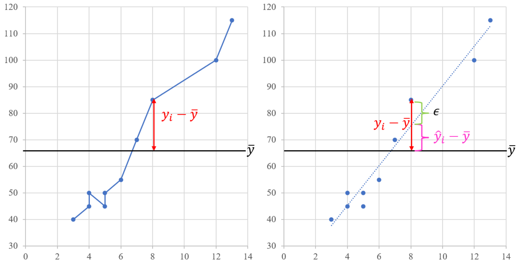
The conventional way of introducing \(F\) test in regression begins with sum of squares decomposition. \[\begin{align*} y_i-\bar{y}&=y_i-\hat{y}_i+\hat{y}_i-\bar{y}\nonumber\\ \sum_{i=1}^{n}(y_i-\bar{y})^2&=\sum_{i=1}^{n}(y_i-\hat{y}_i)^2+\sum_{i=1}^{n}(\hat{y}_i-\bar{y})^2+2\sum_{i=1}^{n}(y_i-\hat{y}_i)(\hat{y}_i-\bar{y})\nonumber\\ \end{align*}\] where \(2\sum_{i=1}^{n}(y_i-\hat{y}_i)(\hat{y}_i-\bar{y})=0\) (see Section 5.2 for proof),

  • \(\sum_{i=1}^{n}(y_i-\bar{y})^2\) is the total sum of squares (SST), represents the total variability of \(y\),
  • \(\sum_{i=1}^{n}(\hat{y}_i-\bar{y})^2\) is the sum of square of regression (SSR), represents the variability of \(y\) that can be explained by \(x_1\), \(\cdots\), \(x_p\),
  • \(\sum_{i=1}^{n}(y_i-\hat{y}_i)^2\) is the sum of square of error (SSE), represents the variability of \(y\) that not explained by \(x_1\), \(\cdots\), \(x_p\).

Then we have the following \(F\) test table:

Source \(df\) Mean squares \(F\)
SSR \(p\) \(MSR=\frac{SSR}{p}\) \(F=\frac{MSR}{MSE}\)
SSE \(n-p-1\) \(MSE=\frac{SSE}{n-p-1}\)
SST \(n-1\)

of which the hypotheses are

  • h0: \(\beta_1\)=\(\beta_2\)=\(\cdots\)=\(\beta_p\)=0,
  • h1: not all \(\beta\)s equal 0.

If we observed a significant \(p\) value for \(F\), we reject the h0. But why are \(df_{SSR}=p\), and \(df_{SSE}=n-p-1\)?

Let’s take a closer look at SST. \(y_i-\bar{y}\) can be viewed as the residual of predicting \(y_i\) using \(\bar{y}\). It is easy to see that \(\bar{y}\) is essentially a multiple regression model as follow \[\begin{align} \hat{y}_i&=\bar{y}+0x_{i1}+0x_{i2}+\cdots+0x_{ip}, \nonumber \end{align}\] of which \(x_1\), \(\cdots\), \(x_p\) are incapable of predicting any variability of \(y\). This is effectively the h0 model as well as the worst model (m2) we can have for now. Thus \(\sum_{i=1}^{n}(y_i-\bar{y})^2\) is the sum of squared residuals of h0 model. To obtain this model, we have to impose \(p\) restrictions onto \[\begin{align} \hat{y}_i&=\hat{\beta}_0+\hat{\beta}_1x_{i1}+\hat{\beta}_2x_{i2}+\cdots+\hat{\beta}_px_{ip}, \nonumber \end{align}\] also known as unrestricted model in the sense that all \(p\) slopes are estimated freely. What is the sum of squared residuals of unrestricted model?

  • SSE: \(\sum_{i=1}^{n}(y_i-\hat{y}_i)^2\).

How much worse is the fit of restricted model comparing to that of unrestricted one?

  • SST-SSE=SSR: \(\sum_{i=1}^{n}(\hat{y}_i-\bar{y})^2\).

But it is hard to tell whether SSR is a big difference, because SSR depends on the scale of \(y\). A comparison of SST to SSE is meaningless unless we account for the scale of \(y\). An intuitive solution would be the relative ratio: \[\begin{align*} \frac{SST-SSE}{SSE}. \end{align*}\] This ratio express how much larger is SST compared to SSE as a percentage. However this ratio leaves sampling uncertainty out of the picture. The larger the sample size, the smaller fluctuation of sample statistics, as well as the standard error of parameter in interest (i.e. \(SE_{\bar{x}}=\sigma/\sqrt{n}\)). Thus, if \((SST-SSE)/SSE=0.5\), implying that the restricted model is 0.5 times (50%) worse than the unrestricted model, this would be considered as a more impressive evidence with a larger sample size than with a smaller one. Because \[\begin{align*} F=\frac{SST-SSE}{SSE}\frac{n-p-1}{p}, \end{align*}\] where \(n-p-1\) magnifies the effect of relative ratio in the sense that a larger \(n\) shall leads to a larger \(F\), if \((SST-SSE)/SSE\) remained unchanged.

But why \(n-p-1\) rather than \(n\)? Because in a data set with \(n\) observations, we have \(n\) pieces of information. When estimating the unrestricted model with \(p+1\) parameters, 1 intercept and \(p\) slopes, we end up using \(p+1\) of the observations available, leaving only \(n-p-1\) pieces of truly independent information.

The last question is why \(p\) in the denominator of the second factor. This is because we want to know the average improvement of unrestricted model per restriction by taking into consideration the fact that larger model with less restrictions could easily enjoy larger SSR due to sampling uncertainty.

set.seed(3817)
n <- 100
p <- 50 # increase from 10 to 50 by 10
y <- 0.5 + rnorm(n)
x <- matrix(rnorm(n * p), n, p)
colnames(x) <- paste0("x", 1:p)
df <- data.frame(x, y)
reg_unrestricted <- lm(y ~., data = df)
reg_restricted <- lm(y ~ 1, data = df)
SSE <- sum(residuals(reg_unrestricted)^2)
SST <- sum(residuals(reg_restricted)^2)
(SST - SSE)/SSE
#> [1] 0.9144509
((SST - SSE)/SSE)*((n - p - 1)/p) # no longer a large value for F(50, 49)
#> [1] 0.8961619
summary(reg_unrestricted)
#> 
#> Call:
#> lm(formula = y ~ ., data = df)
#> 
#> Residuals:
#>      Min       1Q   Median       3Q      Max 
#> -1.54198 -0.39031  0.06124  0.41127  1.90320 
#> 
#> Coefficients:
#>              Estimate Std. Error t value Pr(>|t|)   
#> (Intercept)  0.184604   0.155570   1.187  0.24109   
#> x1          -0.045788   0.125312  -0.365  0.71639   
#> x2           0.206352   0.155552   1.327  0.19080   
#> x3           0.255084   0.121485   2.100  0.04093 * 
#> x4          -0.466889   0.146852  -3.179  0.00256 **
#> x5          -0.065825   0.126515  -0.520  0.60521   
#> x6           0.245485   0.152579   1.609  0.11406   
#> x7           0.316976   0.165448   1.916  0.06123 . 
#> x8           0.141824   0.133262   1.064  0.29243   
#> x9          -0.022508   0.133226  -0.169  0.86654   
#> x10          0.114777   0.161646   0.710  0.48104   
#> x11         -0.101359   0.142906  -0.709  0.48152   
#> x12         -0.242710   0.129101  -1.880  0.06606 . 
#> x13          0.087706   0.133027   0.659  0.51278   
#> x14          0.042302   0.138654   0.305  0.76159   
#> x15         -0.066785   0.155709  -0.429  0.66987   
#> x16         -0.118709   0.135244  -0.878  0.38437   
#> x17         -0.096478   0.152184  -0.634  0.52906   
#> x18          0.160714   0.134774   1.192  0.23882   
#> x19          0.111137   0.149870   0.742  0.46190   
#> x20         -0.190947   0.151706  -1.259  0.21412   
#> x21         -0.009397   0.122639  -0.077  0.93923   
#> x22         -0.011484   0.152991  -0.075  0.94047   
#> x23          0.051981   0.118675   0.438  0.66330   
#> x24          0.034629   0.120958   0.286  0.77586   
#> x25         -0.008070   0.139934  -0.058  0.95425   
#> x26         -0.026887   0.137960  -0.195  0.84629   
#> x27          0.014170   0.130896   0.108  0.91424   
#> x28          0.044710   0.129484   0.345  0.73135   
#> x29          0.146422   0.134778   1.086  0.28262   
#> x30         -0.108739   0.138832  -0.783  0.43725   
#> x31          0.009189   0.143688   0.064  0.94927   
#> x32         -0.025615   0.121197  -0.211  0.83349   
#> x33          0.150368   0.154532   0.973  0.33530   
#> x34         -0.023642   0.135977  -0.174  0.86269   
#> x35         -0.268318   0.141200  -1.900  0.06329 . 
#> x36         -0.122918   0.128102  -0.960  0.34200   
#> x37          0.090454   0.137385   0.658  0.51337   
#> x38          0.134963   0.138404   0.975  0.33428   
#> x39          0.047747   0.137773   0.347  0.73041   
#> x40         -0.186315   0.160376  -1.162  0.25097   
#> x41         -0.118880   0.153887  -0.773  0.44352   
#> x42         -0.016028   0.144216  -0.111  0.91196   
#> x43          0.088327   0.142575   0.620  0.53845   
#> x44         -0.088814   0.134287  -0.661  0.51147   
#> x45         -0.160326   0.151048  -1.061  0.29370   
#> x46          0.149468   0.135273   1.105  0.27458   
#> x47         -0.063921   0.147372  -0.434  0.66638   
#> x48          0.098527   0.137770   0.715  0.47791   
#> x49         -0.035065   0.130644  -0.268  0.78952   
#> x50         -0.002063   0.109886  -0.019  0.98510   
#> ---
#> Signif. codes:  0 '***' 0.001 '**' 0.01 '*' 0.05 '.' 0.1 ' ' 1
#> 
#> Residual standard error: 0.9385 on 49 degrees of freedom
#> Multiple R-squared:  0.4777, Adjusted R-squared:  -0.05535 
#> F-statistic: 0.8962 on 50 and 49 DF,  p-value: 0.6497

Reference: Understanding the F Statistic.

2.2 Likelihood ratio test

Likelihood ratio test (LRT) is one of the most popular test for model comparison in statistics, it is also the foundation of model fit evaluation in SEM.

2.2.1 What is likelihood ratio and likelihood ratio test

In statistics, just like other conventional statistical tests, i.e. t test, anova, LRT is used to test a hypothesis. LRT compares the goodness of fit of a null hypothesis model (h0 model, with less parameters) to that of an alternative model (h1 model, with more parameters). The h0 model is obtained by imposing some constraints over the h1 model (fix parameter at 0), and therefore nested in h1 model (i.e., h0 model is a special case of h1 model).

Suppose we have null hypothesis and alternative hypothesis as following:

  • h0: the parameter \(\theta\) of underlying model is in the parameter space \(\Theta_0\),
  • h1: the parameter \(\theta\) of underlying model is in the parameter space \(\Theta_0^\text{c}\),

where \(\Theta_0^\text{c}\) is the complement of \(\Theta_0\), the entire parameter space \(\Theta = \Theta_0 \cup \Theta_0^{\text{c}}\). The likelihood ratio is given by:

\[\text{LR} =\frac{~ \sup_{\theta \in \Theta_0} \mathcal{L}(\theta)=\mathcal{L}(\hat{\theta}_0)}{\sup_{\theta \in \Theta_o^{\text{c}}} \mathcal{L}(\theta)=\mathcal{L}(\hat{\theta}_1)}\]

where the \(\sup\) notation refers to the supremum and is realized through maximum likelihood estimation, thus \(\hat{\theta}\) represent the maximum likelihood estimator. As all likelihoods are positive, and as the constrained maximum cannot exceed the unconstrained maximum, the likelihood ratio is bounded between zero and one. Based on the ratio of their likelihoods. If the h0 model is true, the h1 model found by maximizing over the entire parameter space should be identical to the h0 model at population level, therefore the likelihood of h0 model should be very close to that of h1 model at sample level, the two likelihoods only differ by sampling error. Thus essentially, the likelihood-ratio test tests whether this ratio is significantly different from one.

Because \(\text{LR}\) is only a ratio and null hypothesis testing relies on an asymptotic sampling distribution of estimator, thus often the likelihood-ratio test statistic is expressed as :

\[\text{T}_\text{LR} =-2\ln(\text{LR})= -2 \left[\ell(\hat{\theta}_0) - \ell( \hat{\theta}_1) \right]\]

where \(\ell(\hat{\theta_0}) = \ln \left[\mathcal{L}(\hat{\theta}_0)\right],\ell( \hat{\theta}) = \ln \left[\mathcal{L}(\hat{\theta}_0)\right]\). \(\ell( \hat{\theta}_1)\)is the logarithm of the maximized likelihood function \(\mathcal{L}\) for sample data, and \(\ell(\hat{\theta}_0)\) is the maximal value in the special case that the null hypothesis is true (but not necessarily a value that maximizes \(\mathcal{L}\) for the sampled data). \(\hat{\theta}_0 \in \Theta_0\) and \(\hat{\theta}_1 \in \Theta_0^{\text{c}}\) denote the respective arguments of the maxima and the allowed ranges they’re embedded in. Multiplying by -2 ensures mathematically that \(\lambda_\text{LR}\) converges asymptotically (if \(n\) goes to infinity) to \(\chi^2\) distribution with degrees of freedom equal to the difference in dimensionality of \(\Theta_0^{\text{c}}\) and \(\Theta_0\), i.e. \(df = \#\text{par}_{h1}-\#\text{par}_{h0}\), if the null hypothesis happens to be true. If the resulting \(\hat{\lambda}_\text{LR}\) is larger than the critical value of \(\chi^2_{df}\), reject h0, otherwise do not reject h0.

The likelihood-ratio test requires that the models be nested. Two models are nested when one model is a special case of the other so that the special case model is considered a reduced model and the model in which the reduced model nested is the full model.

To conduct LRT, the key steps are: specifying h1 model and h0 model and count \(df\).

2.2.2 How to specify h1 model and h0 model?

LRT compares h0 model with h1 model. Normally, we use the best model as h1 model so that if our hypothezied one, h0 model, is true, \(L(\hat{\boldsymbol{\theta}}_1)>L(\hat{\boldsymbol{\theta}}_0)\) and the likelihood of these two model shall only differ slightly by sampling error. Here, best model corresponds to the most complex model available in the modeling framework we use to fit data. H0 model is obtained by imposing restrictions on the most complex model. The number of unknown parameters in h0 model decrease as well as its model complexity.

H0 model is also know as restricted model, whereas h1 model is also know as saturated model, or unrestricted model, due to the fact that it is the most complex model available for fitted data set. The concept of “most complex” could be approached from two different perspectives:

  1. Theoretical perspective.

This is a more general understanding of “complexity”. For example, given 3 \(x\)s and 1 \(y\), we can fit a multiple regression \[y=\beta_0+\beta_1x_1+\beta_2x_2+\beta_3x_3+\epsilon,\] we can also fit a multiple regression with all 3 2nd order interaction effects \[y=\beta_0+\beta_1x_1+\beta_2x_2+\beta_3x_3+\beta_4x_1x_2+\beta_5x_1x_3+\beta_6x_2x_3+\epsilon.\] The latter one is clearly more complex than the former model. However, given this 4 variables scenario, we can actually have a wide variety of choices in terms of complex model. For example, we can fit a even more complex model with non-linear effect \[y=\beta_0+\beta_1x_1+\beta_2x_2+\beta_3x_3+\beta_4x_1x_2+\beta_5x_1x_3+\beta_6x_2x_3+\beta_7x_1^2+\epsilon.\] With so many complex models available, researchers must base their decision on theory, thus the “complexity” of model is purely a theory-driven concept.

  1. Statistical perspective.

This is an understanding that is specific to LRT. The “complexity” of model is capped by the number of variables used, where “variable” refers to background variable in the right hand side of regression model, or column of non-dependent-variable in data set. For example, if we have 3 \(x\)s and 1 \(y\), we decide to fit a model (h0 model) with all interaction effects \[\begin{align*} y &=\beta_0+\beta_1x_1+\beta_2x_2+\beta_3x_3+\\ &\quad \enspace \beta_4x_1x_2+\beta_5x_1x_3+\beta_6x_2x_3+\\ &\quad \enspace \beta_7x_1x_2x_3+\\ &\quad \enspace \epsilon. \end{align*}\] In this case, we have 7 background variables (\(x_1\), \(x_2\), \(x_3\), \(x_1x_2\), \(x_1x_3\), \(x_2x_3\), \(x_1x_2x_3\)) in the right hand side of the model above, 7 columns of non-dependent variables in the data sets to which the model is fitted. We can not increase the complexity of model without adding new background variable to the right hand side of model above or new column into the data set (i.e. add \(x_1^2\)). Thus for LRT, the most complex model in this case is the same model above, that is, h1=h0.

Likewise, it is easy to see that if we decide to fit \[y=\beta_0+\beta_1x_1+\beta_2x_2+\beta_3x_3+\epsilon,\] which is the h0 model, the number of background variables or the number of non-dependent-variable columns is 3. The most complex model available is h0 itself, therefore h1=h0.

What if we want to fit a h0 with less parameter than h1? Suppose we have 2 \(x\)s and 1 \(y\), we decide to use a linear regression without interaction effect (h0 model) \[y_i=\beta_0+\beta_{1}x_{1i}+\beta_{2}x_{2i}+\epsilon_i.\] Then the h1 model is also the h0 model. If we assumed that \(x_2\) has no effect on \(y\), we can fix the slope of \(x_2\) at 0, the resulting h0 model is \[y_i=\beta_0+\beta_{1}x_{1i}+0x_{2i}+\epsilon_i,\] not \[y_i=\beta_0+\beta_{1}x_{1i}+\epsilon_i.\] In this case, there are still 2 background variables or 2 columns of non-dependent variables in data set. Thus the h1 model remains unchanged, the h0 model becomes a smaller one.

Other examples:

2.2.2.1 Coding session

Assume we have a linear regression model with fixed \(x\)s as \[y_i=\beta_0+\beta_1x_{1i}+\beta_2x_{2i}+\beta_3x_{3i}+\epsilon_i,\]

In this scenario, we can have the following models available for testing:

  • m1: \(y=\beta_0+\beta_1x_1+\beta_2x_2+\beta_3x_3+\epsilon_i\),
  • m2: \(y=\beta_0+\beta_1x_1+\beta_2x_2+0x_3+\epsilon_i\)
  • m3: \(y=\beta_0+\beta_1x_1+0x_2+0x_3+\epsilon_i\)

Task 1

Data generation model is m2 and: \(\beta_0=\beta_1=\beta_2=1\), \(\beta_3=0\), \(\epsilon_i\in N(0,1)\).

  1. Generate data from this model with sample size \(n=1000\),
  2. Fit m1, m2, and m3 using Mplus (the equivalent R function lm() in R) separately,
  3. Conduct LRT using Mplus to compare m2 (h0) with m1 (h1), m3 (h0) with m1 (h1), and m3 (h0) with m2 (h1), record the resulting p-value (the equivalent R function is lmtest::lrtest(),
  4. Replicate steps 1-3 100 times, count the number of p-value < .05 (R learner only).

For non-quant students, do steps 2-3 using “1y 3xs no interaction.txt”.

Task 2

Data generation model is m3: \(\beta_0=\beta_1=1\), \(\beta_2=\beta_3=0\), \(\epsilon_i\in N(0,1)\). Repeat steps 1-4.

For non-quant students, do steps 2-3 using “1y 3x 2ind_x no interaction.txt”.

Task 3

Assume we have the following linear regression model with fixed \(x\)s as data generation model \[\begin{align*} y_i&=\beta_0+\beta_1x_{1i}+\beta_2x_{2i}+\beta_3x_{3i}+\\ &\quad \enspace \beta_4x_{1i}x_{2i}+\beta_5x_{1i}x_{3i}+\beta_6x_{2i}x_{3i}+\\ &\quad \enspace \beta_7x_{1i}x_{2i}x_{3i}+\\ &\quad \enspace \epsilon_i, \end{align*}\] where \(\beta_0=\beta_1=\beta_2=\beta_3=\beta_4=\beta_7=1\), \(\beta_5=\beta_6=0\), \(\epsilon_i\in N(0,1)\).

In this scenario, we can have the following models available for testing:

  • m1, with all 2nd and 3rd order interaction effects:

\[\begin{align*} y_i&=\beta_0+\beta_1x_{1i}+\beta_2x_{2i}+\beta_3x_{3i}+\\ &\quad \enspace \beta_4x_{1i}x_{2i}+\beta_5x_{1i}x_{3i}+\beta_6x_{2i}x_{3i}+\\ &\quad \enspace \beta_7x_{1i}x_{2i}x_{3i}+\\ &\quad \enspace \epsilon_i, \end{align*}\]

  • m2, remove 2 2nd order interaction effects:

\[\begin{align*} y_i&=\beta_0+\beta_1x_{1i}+\beta_2x_{2i}+\beta_3x_{3i}+\\ &\quad \enspace \beta_4x_{1i}x_{2i}+0x_{1i}x_{3i}+0x_{2i}x_{3i}+\\ &\quad \enspace \beta_7x_{1i}x_{2i}x_{3i}+\\ &\quad \enspace \epsilon_i, \end{align*}\]

  • m3, all 3 2nd order interaction effects, no 3rd order interaction effect:

\[\begin{align*} y_i&=\beta_0+\beta_1x_{1i}+\beta_2x_{2i}+\beta_3x_{3i}+\\ &\quad \enspace \beta_4x_{1i}x_{2i}+\beta_5x_{1i}x_{3i}+\beta_6x_{2i}x_{3i}+\\ &\quad \enspace 0x_{1i}x_{2i}x_{3i}+\\ &\quad \enspace \epsilon_i, \end{align*}\]

  • m4, no interaction:

\[\begin{align*} y_i&=\beta_0+\beta_1x_{1i}+\beta_2x_{2i}+\beta_3x_{3i}+\\ &\quad \enspace 0 x_{1i}x_{2i}+ 0 x_{1i}x_{3i}+ 0 x_{2i}x_{3i}+\\ &\quad \enspace 0 x_{1i}x_{2i}x_{3i}+\\ &\quad \enspace \epsilon_i, \end{align*}\]

  1. Generate data from this model with sample size \(n=1000\),
  2. Fit m1, m2, and m3 using Mplus (the equivalent R function lm() in R) separately,
  3. Conduct LRT using Mplus to compare m2 (h0) with m1 (h1), m3 (h0) with m1 (h1), and m4 (h0) with m1 (h1), record the resulting p-value (the equivalent R function is lmtest::lrtest()),
  4. Replicate steps 1-3 100 times, count the number of p-value < .05 (R learner only).

For non-quant students, do steps 2-3 using “1y 3xs interaction.txt”.

2.2.3 Model misspecification

LRT is able to detect model misspecification of h0 model only when:

  1. h1 model is correctly specified,
  2. h0 is nested in h1.

There are basically three types of model misspecifications.

  1. Parameter-level misspecification
  • non-existing parameter being estimated freely: h0 model has superfluous parameter of which the population value is 0 (e.g. true model is m3 but fit model is m2);
  • existing non-zero parameter being fixed (usually at 0): h0 model lacks parameter of which the population value is non-zero (e.g. true model is m2 but fit model is m3).

For the first type of parameter-level misspecification, LRT shall endorse the h0 model with superfluous parameters by generating a p-value > 0.05, because 0 is within the parameter space of h0 when freely estimated. In this case, if we continued to fix superfluous parameter at 0 to obtain a new smaller h0 model, then LRT shall endorse this new h0 model without superfluous parameter as well.

For the second type of parameter-level misspecification, LRT shall reject the h0 model by generating a p-value < 0.05, because when fixing an existing parameter at 0, the parameter space of this specific parameter is 0 and does not include the true value (non-zero), h0 is false.

  1. Function-level misspecification:

The regression relationship between two variables is not linear, but a linear regression is used to fit the data. \[\begin{align*} \text{True model: }y=f(x)&=\beta_0+\beta_1x^2,\\ \text{Fitting model: }y&=\beta_0+\beta_1x. \end{align*}\]

Function-level misspecification usually leads to non-nest models and is beyond the capability of LRT. Because normally we fit linear model to data, h0 and h1 model shall all be linear. Thus there will be model misspecification in both h0 and h1 models, the asymptotic distribution of LRT test statistic will be violated.

  1. Distribution-level misspecification

In general, if we use maximum likelihood, we assume to have normally distributed data. However, this distributional assumption may not be hold in real data. If violated, even if we fit the true model using normal-based ML, we shall still have biased parameter estimation. Therefore distribution-level misspecification is always beyond LRT.
2.3 Model fit indices

After fitting a specified model to data, we answer the question “how good is our model” by model-data fit. Model fit indices abound, most of them are directly based on likelihood ratio test (LRT).

2.3.1 The best model and the worst model

In regression, the best model we can fit to data is the h1 model, that is the saturated model/unrestricted model. Saturated means no extra parameter can be added to the existing model, \(df\) of the LRT is 0.

The worst model we can fit to data is the baseline model/null model. In this model, the variation of \(y\) can no be explained by any \(x\). For example, for a regression model with 2 \(x\)s, the the baseline model/null model is

\[y=\beta_0+0x_1+0x_2\]

2.3.2 LRT-based model fit indices: incremental measure of fit

The LRT test statistics of tested model (h0 model) asymptotically follows \(\chi^2\) distribution with \(df=\#\text{par}_{h1}-\#\text{par}_{h0}\).

2.3.2.1 Comparative Fit Index and Tucker Lewis Index

\[\begin{align*} \text{CFI}=1-\frac{\max(\text{T}-df,0)}{\max(\text{T}_0-df_0,\text{T}-df)}, \end{align*}\] where \(\text{T}_0\) is test statistics of LRT of null model, and \(df_0=\#\text{par}_{h1}\). CFI measures the extent that h0 model improves compared with the null model. It is restricted between 0 and 1.

\[\begin{align*} \text{TLI/Non-normed Fit Index, NNFI}=1-\frac{df_0}{df}\left(\frac{\text{T}-df}{\text{T}_0-df_0}\right). \end{align*}\] TLI adds penalty for complex model, thus tend to endorse model with less parameters, CFI and TLI should be very close to each other. If the CFI is less than one, then the CFI is always greater than the TLI, only one of the two should be reported to avoid redundancy. But TLI could exceed 1 under certain condition, if so, it is capped at 1 in popular stats software, except for Mplus.

For CFI and TLI

  • \(>0.95\) indicates good model-data fit
  • \(>0.9\) indicates acceptable model-data fit

2.3.2.2 Root Mean Square Error of Approximation

\[\begin{align*} \text{RMSEA}=\sqrt{\frac{\text{T}-df}{df(n-1)}}. \end{align*}\] RMSEA measures the average model misfit per \(df\). It is always positive. Just like TLI, RMSEA tends to endorse small-size model. There is greater sampling error for small \(df\) and low \(n\) models, especially for the former. Thus, models with small \(df\) and low \(n\) can have artificially large values of the RMSEA. For instance, a \(\text{T}\) of 2.098 (a value not statistically significant), with a \(df\) of 1 and \(n\) of 70 yields an RMSEA of 0.126. For this reason Kenny & Kaniskan (2014) argue to not even compute the RMSEA for low \(df\) models.

A confidence interval can be computed for the RMSEA. Its formula is based on the non-central \(\chi^2\) distribution and usually the 90% interval is used. Ideally the lower value of the 90% confidence interval includes or is very near zero (or no worse than 0.05) and the upper value is not very large, i.e., less than 0.08 or perhaps a 0.10. The width of the confidence interval can be very informative about the precision in the estimate of the RMSEA.

  • \(\text{RMSEA}\leq 0.05\) indicates a close fit of a model
  • \(\text{RMSEA}\leq 0.08\) indicates a reasonable model
  • \(\text{RMSEA}>1\) indicates a bad model

CFI, TLI and RMSEA treat \(\text{T}=df\) as the best possible model.

2.3.2.3 Standardized Root Mean Square Residual

I have no idea what is the formula of SRMR for regression in Mplus. I only know that SRMR is an absolute measure of fit based on residual and has no penalty for model complexity.

  • \(\text{SRMR} = 0\) indicates perfect fit
  • \(\text{SRMR} < .08\) is generally considered a good fit (Hu & Bentler, 1999).

Reference: SRMR in Mplus.

2.3.3 Non-LRT-based model fit indices: comparative measure of fit

Following are several non-LRT-based model fit indices: Akaike Information Criterion (AIC), Bayesian Information Criterion (BIC), and sample-size adjusted BIC (SABIC)

\[\begin{align*} \text{AIC}&=-2\log(L)+2q\\ \text{BIC}&=-2\log(L)+\log(n)q\\ \text{SABIC}&=-2\log(L)+\log(\frac{n+2}{24})q, \end{align*}\] where \(q\) is the number of estimated parameters in the model. Because AIC and BIC have no fixed scale, no cut-off value is available.

Lower values of AIC indicate a better fit and so the model with the lowest AIC is the best fitting model. There are somewhat different formulas given for the AIC in the literature, but those differences are not really meaningful as it is the difference in AIC that really matters. The AIC makes the researcher pay a penalty of two for every parameter that is estimated.

BIC increases the penalty as sample size increases. The BIC places a high value on parsimony. The SABIC or SABIC like the BIC places a penalty for adding parameters based on sample size, but not as high a penalty as the BIC.

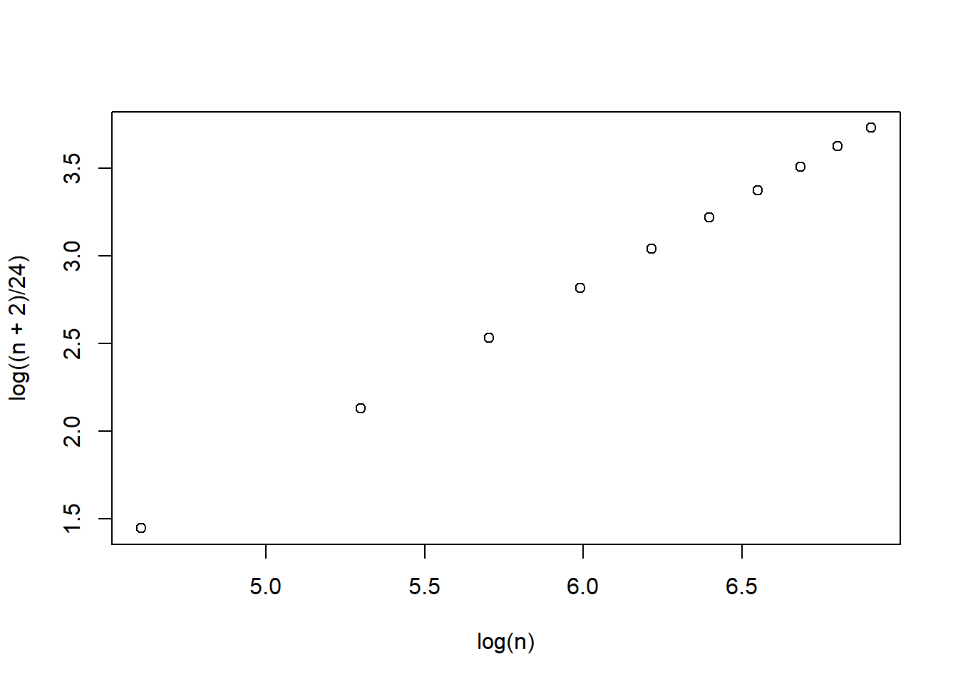
n <- seq(100, 1000, 100)
plot(log(n), log((n + 2)/24))

2.3.4 Model comparison

There are two types of model comparison:

  • nested model comparison,
  • unnested model comparison,

Nested model comparison is usually conducted using LRT-based \(\chi^2\) difference test.

A model can be seen as a special case of another by imposing constraints (force to be 0) on parameters. If the model fit of a complex model was good, then constraints can be set to test the resulting simpler model.

\[\Delta_{\text{T}}=\text{T}_{\text{simpler}}-\text{T}_{\text{larger}}\] If \(\Delta_{\text{T}}\) is significant, then the constraints are not appropriate. Otherwise, the simpler model can be used.

Unnested model comparison is usually conducted using fit indices.

2.3.4.1 Coding session

Compare m1, m2, m3, m4 using LRT-based model fit indices.