5.2 Realized measures of volatility
- In the theory it is commonly assumed that dynamics of log prices \(p_t=\ln(P_t)\) follow a continuous stochastic diffusion process known as an Ito process
\[\begin{equation} dp_t=\mu_t dt+\sigma_t dW_t \end{equation}\]
where \(\mu_t\) is the drift, \(\sigma_t\) is a variance (diffusion) process and \(W_t\) is a Wiener process (standard Brownian motion, with independent and stationary increments and also independent from variance process \(\sigma_t\))
- By taking the integral over a one day interval \([t,~~t-1]\), and after some rearrangements a daily integrated variance (IV) is given as
\[\begin{equation} IV=\int_{t}^{t-1} \sigma^2_t\,dt \end{equation}\]
From above notation, an integrated variance is usually understood as quadratic variation of semi–martingale process, and it is unknown quantity which can be estimated using discrete prices observed in a very short time intervals
The simplest way to estimate daily IV is the cumulative sum of squared equidistant intraday returns sampled at interval \(\Delta\), which is known as realized volatility (RV)
\[\begin{equation} RV^{\Delta}_t=\sum_{j=1}^m r^2_{t,j} \end{equation}\]
- RV is realized measure of IV, and it converges in probability to the quadratic variation of the semi–martingale process when the number of intraday returns \(m\) increases indefinitely
\[\begin{equation} \lim_{m \to \infty}\sum_{j=1}^m r^2_{t,j} \xrightarrow{P} \int_{t}^{t-1} \sigma^2_t\,dt \end{equation}\]
Equation (6.43) implies that one would use as many intraday returns as possible to compute the daily realized volatility. In practice, this means using the tick–by–tick or high–frequency prices
Intraday returns observed at the finest possible interval are contaminated with microstructure noise (such as bid–ask bounce, nonsynchronous trading, etc.), which makes RV biased estimate of the true IV. As a matter of fact, the RV becomes more biased as the sampling interval \(\Delta\) decreases (or sampling frequency increases), i.e. \(\lim_{\Delta \to 0}\) when \(\lim_{m \to \inf}\)
There are two methods commonly used in the literature to handle the microstructure noises in calculating RV. The first method is used to obtain an optimal sampling interval \(\Delta^{*}\) (by minimizing MSE a compromise between efficiency and biasness can be achieved)
For heavily traded stocks, the optimal interval is often between \(1\) to \(5\) minutes, and for less liquid stocks (characterized by infrequent trading at under–developed or emerging markets) the optimal interval is between \(5\) do \(30\) minutes (the cost of sparse sampling is a high variance of an estimator – inconsistency – as a small number of observations is left for computational reasons)
The second method to calculating realized volatility is to use subsampling technique and to correct the bias, which results in two–times scale realized volatility (TTSRV)
\[\begin{equation} TTSRV_t = \underbrace{\left( 1 - \dfrac{\bar{n}}{m} \right)}_{sample~~adjustment} \left( \underbrace{RV^{ave}_t}_{\substack{RV~~at \\ slow~~scale}} - \underbrace{\dfrac{\bar{n}}{m} \underbrace{RV^{\Delta}_t}_{\substack{RV~~at \\ fast~~scale}}}_{bias~~correction} \right) \end{equation}\]
- TTSRV uses all the prices (data are not throw away) and still have unbiased and consistent estimator of the integrated variance because it uses the highest possible sampling frequency \(J\) (fast time scale) to filter out the magnitude of the noise term by subtracting it from the average RV at a sparse frequency \(K\) (slow time scale)
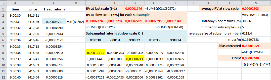
FIGURE 5.1: Example of TTSRV calculation at fast scale of 1 second and slow scale of 5 seconds
If the fast scale frequency \(J\) is set in advance (as the highest sampling frequency at which we can eliminate zero prices and transaction gaps within equidistant and non–empty intervals), the major problem that remains is to determine an optimal slow scale frequency \(K^{*}\). The optimal slow time scale (the optimal number of subsamples) can be found by minimizing the mean squared error (MSE) of the average sparse RV.
Not only the microstruture noise contaminates realized volatility, but also price jumps, and therefore a price jumps robust estimator are proposed in the litearture
Bipower variation (BPV) is realized volatility obtained as the sum of the product between absolute adjacent intraday returns, which damps the jump impact if even occurs for sufficiently small \(\Delta\)
\[\begin{equation} BPV^{\Delta}_t=\dfrac{\pi}{2}\sum_{j=2}^m |r_{t,j}||r_{t,j-1}| \end{equation}\]
- Similar to \(BPV^{\Delta}_t\), two estimators also emerged in the literature, i.e. minimized and medianized realized volatility
\[\begin{equation} \begin{aligned} MinRV^{\Delta}_t&=\dfrac{\pi}{\pi-2}\dfrac{m}{m-1} \\ MedRV^{\Delta}_t&=\dfrac{\pi}{6+\pi-4\sqrt{3}\}\dfrac{m}{m-2}\sum_{j=1}^{m-1}med(|r_{t,j-1}|,|r_{t,j}|,|r_{t,j+1}|)^2 \end{aligned} \end{equation}\]
Both estimators \(MinRV^{\Delta}_t\) and \(MedRV^{\Delta}_t\) follow a concept of the nearest neighbor truncation by the use of the minimum operator on blocks of two returns and the median operator on blocks of three returns, and they have better performance in the finite samples compared to the \(BPV^{\Delta}_t\)
As previously highlighted, \(RV^{\Delta}_t\) is robust to microstructure noise as well as \(TTSRV^{\Delta}_t\) depending on the parameters \(\Delta\) and \(K\), while \(BPV^{\Delta}_t\), \(MinRV^{\Delta}_t\) and \(MedRV^{\Delta}_t\) are robust to price jumps only
Robust estimators of IV have also been designed in the presence of both jumps and noise, in particular, robust version of two–times scale realized volatility (RTTSRV), which requires one additional parameter \(\theta\) as a threshold with respect to indicator function. If returns are larger than three standard deviations from the mean (\(\theta=9\)), the indicator function has value 0 and 1 otherwise.