Chapter 6 Lecture 2017-01-24

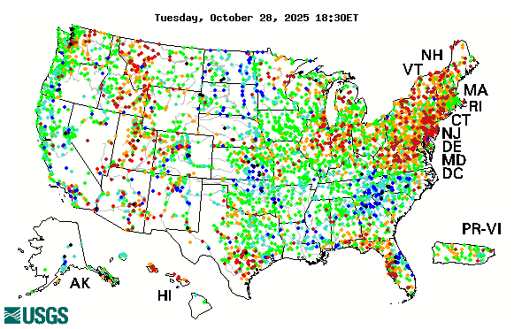
6.1 Environmental Data

6.1.1 Data Science

6.1.2 Why Write a Computer Program?

Accurate and fast math
Written record of what you’ve done
Facilitate collaboration
Change parameters and re-run
Repeatable analysis
Reproducible science?

Ultimately writing a script will save you time and help you do better work

6.1.3 Today: R Computing

Today we’ll cover a “breathless tour” of R and some useful packages. For HW1, you will go on Data Camp and practice these ideas in an interactive setting where you get feedback.

You don’t need to remember specific commands from today
You should remember what is possible and why we might want to do it

We’ll save ~30 minutes for an in-class exercise. We almost certainly won’t get through all these slides – use them as a reference!

Slides will be posted – no need to write down every command. Ask questions!

6.2 Getting Started with R

6.2.1 R: Base plus Packages

“Base” R essential to know but has limited functionality. Packages add specific functionality:

“An R package is a collection of functions, data, and documentation that extends the capabilities of base R. Using packages is key to the successful use of R”
- R4DS

Stored on Central R Archive Network (CRAN)
install.packages()
library() or better yet require()
Many packages with overlapping goals $\rightarrow$ many ways to do the same thing

6.2.2 Arithmetic

We use the +, -, * and / operators. Exponents happen with ^ and modulo with %%. R follows PEMDAS and you can use parentheses ()

5 * (1 - 3)^2

## [1] 20

28%%6

## [1] 4

6.2.3 Assignment Best Practices

Use <- when you’re defining a variable (= works but is not recommended)
Use = inside a function

x <- runif(n=10, min=0, max=1)
y = x + 1 ## SAME EFFECT BUT CONFUSING

6.2.4 Character Data

Not all data has to be numeric.

station_name <- 'Red River of the North at Fargo, ND'
class(station_name)

## [1] "character"

Many functions only take a specific kind of data

sin(station_name)

## Error in sin(station_name): non-numeric argument to mathematical function

6.2.5 Boolean Data

Use == for is equals to; use & for AND; use | for OR.

station_name == 'Missouri River'

## [1] FALSE

(11 > 5) | ('red' == 'blue')

## [1] TRUE

6.2.6 Vectors

Vectors are all the same data type. We create them with c() function for concatenate

numeric_vector <- c(1, 10, 49)
character_vector <- c("a", "b", "c")
boolean_vector <- c(TRUE,FALSE,TRUE)

Numerical operations work element-by-element on vectors

numeric_vector ^ 2

## [1]    1  100 2401

6.2.7 Vector Selection

We select data from a vector using element-wise indexing (starting at 1):

numeric_vector[2]

## [1] 10

We can also use this to sub-set:

x <- 1:21
x[which(x %% 3 == 0)]

## [1]  3  6  9 12 15 18 21

6.2.8 List Data

Each element of a list can have any data type (including other lists)

TA <- list(name = 'James', UNI ='jwd2136', mental_age = 3, 
           is_nice = FALSE, idk = c(2, 3, 5, 7, 11))

We access them with the $ operator

TA$is_nice

## [1] FALSE

6.2.9 Matrices

X <- matrix(1:4, nrow=2, ncol=2)
y <- matrix(5:6, nrow=2, ncol=1)
X

##      [,1] [,2]
## [1,]    1    3
## [2,]    2    4

We can select matrix elements

X[2, 1]

## [1] 2

6.2.10 Matrix Math

To multiply matrices we use %*% and to transpose them we use ^T. To invert a matrix, strangely, we use solve()

\[ \left( X^T X \right)^{-1} X^T y \] is written as

solve(X %*% X^T) %*% X^T %*% y

##      [,1]
## [1,]   -1
## [2,]    2

6.2.11 Data Frames

Data Frames and their extensions are the core of most R data analysis and where R excels. Think spreadsheet: each row is an observation and each column is a variable. For a data frame, each column is a vector (same data type) but a data frame can have columns of different data types

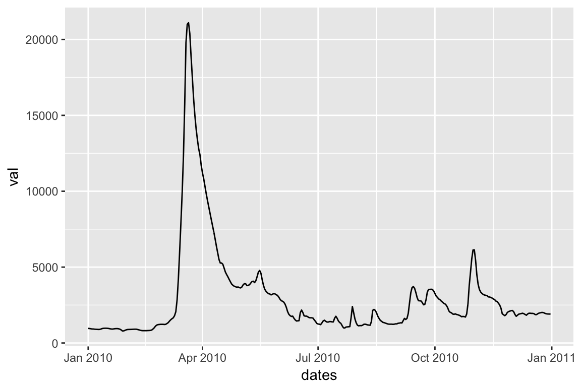
require(waterData)
sflow <- importDVs("05054000", sdate="2010-01-01", edate="2010-12-31")
head(sflow)

##      staid val      dates qualcode
## 1 05054000 961 2010-01-01        A
## 2 05054000 954 2010-01-02        A
## 3 05054000 939 2010-01-03        A
## 4 05054000 922 2010-01-04        A
## 5 05054000 921 2010-01-05        A
## 6 05054000 910 2010-01-06        A

6.2.12 Tibble

We’ll use tibble rather than data.frame structures because they have a few useful extensions. Anything that works for a data.frame works for a tibble. We can turn a data.frame into tibble

sflow <- as_tibble(sflow)
sflow

6.2.13 Creating Data Frames

We can read them from file or specify them by writing each column as a vector

df <- tibble(
  name = c('You', 'Someone', 'Someone Else'),
  grade = c('A+', 'C-', 'F')
)
df

6.2.14 Defining Functions

$f(x) = \sin^2(x)$:

SinSq <- function(x){
  return(sin(x^2))
}

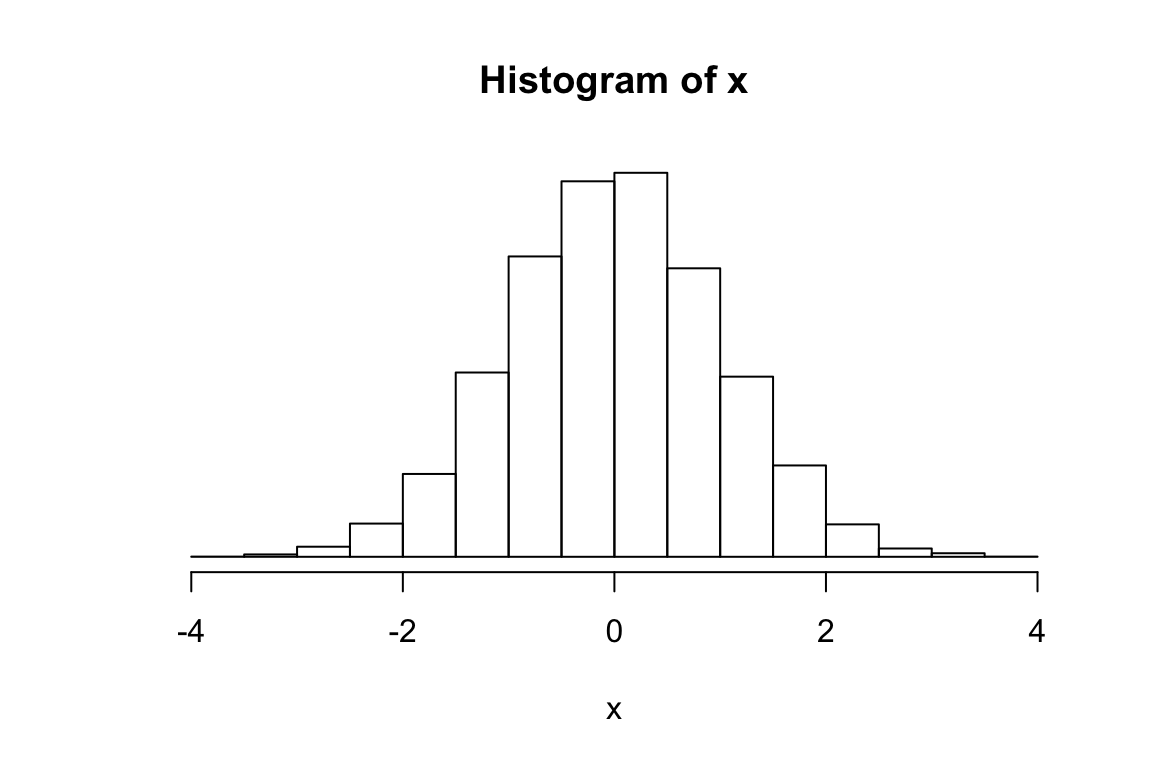
Make pretty histograms:

better_hist <- function(x, ...){
  hist(x, yaxt="n", ylab="", freq=FALSE, ...)
}

6.3 Statistical Computing

6.3.1 Generate Random Numbers

We use the rnorm, rbinom, rexp (see the pattern?) functions.

better_hist(rnorm(n = 10000))

6.3.2 Get the PDF

x <- seq(0, 1, length.out = 1000)
binom_pdf <- dbinom(x=50, size=63, prob=x)
plot(x, binom_pdf, type='l', lwd=3, col='red',
     main='Binomial PDF with 50 Success and 13 Fail')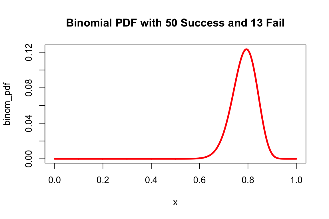

6.3.3 Other Functions

pnorm, pbinom, etc: CDF
qnorm, qpois, qexp etc: inverse CDF
exp, log, log10, sin, cos, etc

See http://seankross.com/notes/dpqr/ for more explanation and comparison

6.3.4 For Loops

They’re slow but useful – for example for bootstrap. For example, if we have 50 observations and want to estimate uncertainty in the mean:

dissolved_oxygen <- exp(rnorm(n=50, mean=2, sd=0.5))
boot_means <- rep(NA, 2500) ## Initialize
for (i in 1:length(boot_means)){ ## loop through
  boot_data <- sample(dissolved_oxygen, length(dissolved_oxygen), 
                      replace=TRUE)
  boot_means[i] <- mean(boot_data) 
}

6.3.5 For Loops and Density Plots

better_hist(boot_means, main='Boostrapped Sample Means')
abline(v=exp(2 + 0.5^2 / 2), lwd=3, col='red', lty=2)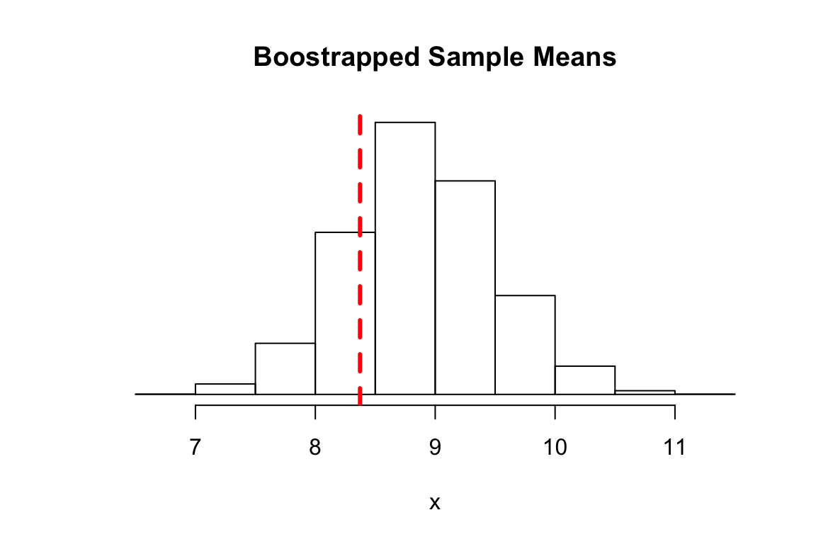

6.4 Data Wrangling

6.4.1 Tidy Data

Easy to work with
Each row is an observation, each column is a variable
Think spreadsheet
Lots of data is not tidy and you have to tidy it: reshape2 and tidyr packages
We’ll make it easy for you this semester

6.4.2 The `dplyr` Package

Reduce operations on tibble objects to simple verbs:

select() select columns
filter() filter rows
arrange() re-order or arrange rows
mutate() create new columns
summarise() summarise values
group_by() allows for group operations in the “split-apply-combine” concept

6.4.3 Pipe Operator

The %>% operator lets us chain together long commands

max(diff(rnorm(1000)))

## [1] 5.223517

rnorm(1000) %>% diff() %>% max()

## [1] 4.362273

6.4.4 For Example

sflow %>%
  mutate(is_spring = lubridate::month(dates) %in% c(3, 4, 5)) %>%
  group_by(is_spring) %>%
  summarize(mean = mean(val), median=median(val))

6.4.5 Visualization

ggplot(sflow, aes(x=dates, y=val)) +
  geom_line()

6.4.6 DF to Vector

We can access elements of a data.frame or tibble with $ operator

mean(sflow$val)

## [1] 3004.838

for complicated chains the pull() function can be useful

sflow %>% pull(val) %>% mean()

## [1] 3004.838

6.5 Next Steps

6.5.1 Get Practicing

6.5.2 Your Courses

Intro to R and tidyverse
Data manipulation with dplyr
Visualization with ggplot2
Reporting with R Markdown so you can create analyses (like homeworks!)

6.5.3 RStudio

To write R you need a text editor on your computer and the R program installed. RStudio is a IDE which lets you run code line by line, see results, format correctly, and more. Highly recommended (though not strictly required) for the course.

6.6 Appendix

6.6.1 Some Best Practices

Write functions!
Use descriptive variable names: flow_cfs $>$ flow $>$ y uusually
A style guide makes your code easier for you to read
Do data exploration in R Markdown files so you can explain what you are doing as you do it!
Code quality will be a [small! ~10%] part of grade for data analysis homeworks

6.6.2 Other Ways to Learn R

Read my HW solutions
Work in groups & read your classmates’ code
Syllabus has some suggested blogs and twitter handles to follow – read the code & analysis of experts
Stay positive!