Chapter 2 Review and Background Information
This course assumes introductory exposure to linear algebra, probability, and calculus. This section will give you a chance to review some topics and refresh your thinking on this subject. You may find some of the following aides to be helpful:
- Zico Kolter’s brief review of Linear Algebra (http://cs229.stanford.edu/section/cs229-linalg.pdf) is useful for anyone who has seen linear algebra but needs some review
- Joe Blitzstein’s Harvard course (http://projects.iq.harvard.edu/stat110) has lecture notes and practice problems for an in-depth look at introductory probability
- Naresh Devineni’s Data Analysis classroom blog (http://www.dataanalysisclassroom.com/) has short lessons (blog posts) on a variety of topics related to statistics and data analysis. It’s recommended to start from the beginning.
- Hadley Wickham’s R for Data Science (http://r4ds.had.co.nz/) is a useful and hands-on guide to R
2.1 Types of Variables and Data
- discrete or categorical variables can take only integer values or are classified into categories
- continuous variables can take any value, with restrictions (positive, between 0 and 1, etc.)
- censored data is observed up to some precision, e.g. we may know values only above or below some threshold, so the data is recorded as a value or a non-detect (value above or below threshold)
2.2 Probability as a relative frequency or a percent chance of occurrence
- Sample observations are independent and identically distributed (drawn from the same population)
- There is an underlying ``law’’ or generating mechanism that governs the relative frequencies of different categories or values, e.g., Binomial or Normal distribution
- Probability is defined as the relative frequency or percent of time an event is expected to occur
- For discrete or categorical events we can associate a probability for each category or value
- For continuous variables, we consider a probability density, which reflects the relative likelihood at any value. The probability of seeing exactly a particular value is 0, since there are infinite such values and the total probability (sum of the chance of all outcomes) needs to equal one. In this case we can define the probability over an interval, \(a \leq x \leq b\), as the area under the probability density function under that interval.
2.3 Some Examples
Given the relative frequency definition of probability, do we need a process to be random to estimate a probability distribution for its values? Consider
- the tosses of 2 pairs of dice, and the outcomes associated with them. Write down each number that can come up by adding the two dice together and the probability of it occurring in a single toss of the doss.
- a perfectly sinusoidal seasonal cycle in temperature with a period of let us say 360 days – assume that the temperature goes from -10 to 10 degrees over the course of the 360 day year. Can you write down a probability (relative frequency) distribution for the temperature data?
For either part you can consider either deriving the probabilities from first principles of actually taking the data and estimating the probabilities of interest using a histogram approach and a very large sample. The following code and plots are in R, which we will start learning soon.
First we generate our simulations of the dice
number_draws <- 10000
dice_1 <- sample(1:6, number_draws, replace = TRUE)
dice_2 <- sample(1:6, number_draws, replace = TRUE)
dice_sum <- tibble(index = 1:number_draws, dice_sum = dice_1 + dice_2)
We can plot the probability of occurrence of each number:
dice_sum %>%
  group_by(dice_sum) %>%
  summarize(p_occurrence = n() / number_draws) %>%
  ggplot(aes(x = dice_sum, y=p_occurrence)) +
  geom_bar(stat='identity') +
  scale_x_continuous(breaks=2:12)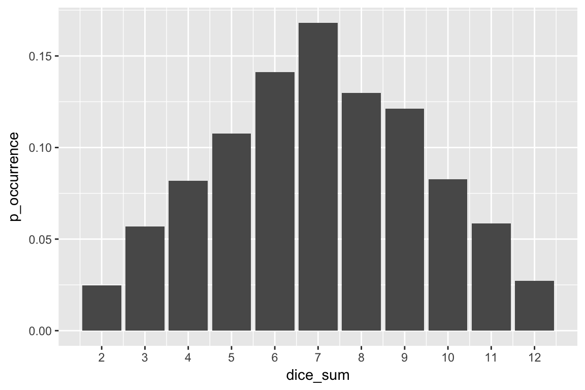
Now we simulate our temperature data. We can plot it as a time series:
number_years <- 10
temp <- tibble(time = 1:(360 * number_years)) %>%
  mutate(temperature = 10*sin(time * pi / 180))
ggplot(temp, aes(x=time, y=temperature)) +
  geom_line()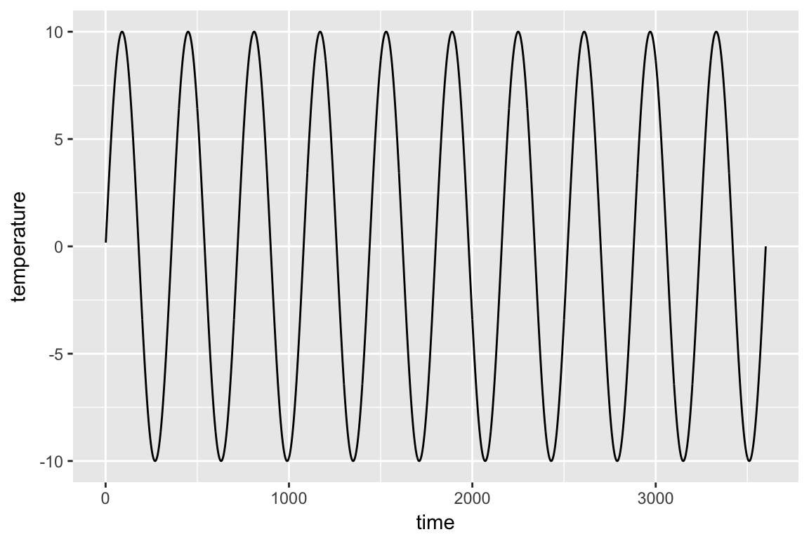
However, we can also view it as a histogram:
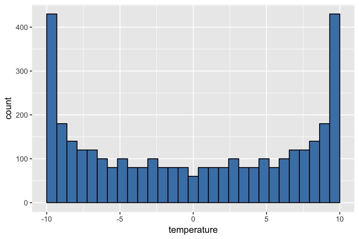
Now comment on/think about the difference in the 2 situations. Arguably, the first case is a random process, and the second is a deterministic process. Yet we compute relative frequency or probability distributions in both cases. How do you interpret this?
2.4 Independence
Two events are independent if the probability of event A does not depend on whether or not event B has happened. Mathematically, this is \[\begin{equation} p(A) = p(A | B) \tag{2.1} \end{equation}\] A key property of independent events is that the joint probability (i.e. probability that both will occur) of independent events is the product of their individual probabilities.
Exercise 2.1 Are successive values of the sine wave in the example above independent? If you know that the current value of the temperature is 0, what is the probability distribution of the next value?
We can answer this question in a fairly straightforward manner by looking at all the times when the temperature was 0 and viewing the distribution of the following day’s temperature:
temp %>%
  mutate(lag_temp = lag(temperature, n=1)) %>%
  drop_na() %>%
  filter(abs(lag_temp) < 0.02) %>%
  ggplot(aes(x = temperature)) +
  geom_histogram(bins=50) +
  labs(x = "Temperature of Subsequent Day",
       title = "When Temperature = 0, What is Next Day's Temperature?")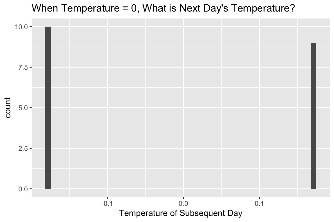
Clearly, there are only two outcomes. We can go a step farther and examine what happens if we look at two lags
temp %>%
  rename(t = temperature) %>%
  mutate(t_plus_1 = lag(t), t_minus_1 = lead(t, 1)) %>%
  drop_na() %>%
  ggplot(aes(x = t_minus_1, y = t)) +
  geom_point(aes(color = t_plus_1)) +
  scale_color_viridis()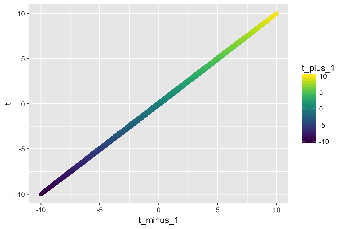
If you figured out what was going on when we looked back only one value it should be pretty clear that if I know \(y_t\) and to \(y_{t-1}\), I completely know \(y_{t+1}\).
Exercise 2.2 If A and B are independent, is A useful for predicting B (or the other way around)? What if they are dependent?
2.5 Mutual Exclusion
If a set of events is complete (all possibilities for the process are covered) and mutually exclusive (i.e., if one occurs the other cannot occur), then the sum of their probabilities is 1. More generally the probabilities of mutually exclusive events can be added.
For another exmample, let’s imagine that we have data on the concentration of Arsenic in well in Bangladesh over a 5 year period. Say we have 100 observations and the events are:
- \(A\): Concentration in the range 0 to 5 ug/l, and
- \(B\) Concentration in the range 5 to 50 ug/l
2.6 Bayes Rule and Dependence
Bayes rule is defined in (2.2): \[\begin{equation} p(A | B) = \frac{p(A, B)}{p(B)} \tag{2.2} \end{equation}\]
Exercise 2.4 Look up Bayes rule give an example of its application
Say we are investigating the concentration of particulate matter in the air in metropolitan areas. We have collected data from \(n=100\) cities. Consider 2 equally spaced population categories between 0 and 10 million. It turns out that approximately 80 cities fall in the first category, i.e., the probability of finding a city with 0 to 5 million people is 0.8, and of 5 to 10 million is 0.2. For category 1 cities, 60 meet the EPA criteria for particulates. For category 2 cities, 10 meet the EPA criteria.
To think of this as a Bayes rule problem, event \(A\) has 2 values (small or large city) and event \(B\) has 2 categories (pass or fail EPA criteria). Let’s organize this information:
bayes_df <- tibble(A = c('small', 'small', 'large', 'large'),
                   B = c('pass', 'fail', 'pass', 'fail'),
                   count=c(60, 20, 10, 10))
bayes_df %>%
  ggplot(aes(x=A, y=B)) +
  geom_tile(aes(fill=count)) +
  geom_text(aes(label=count), color='black') +
  scale_fill_distiller(palette='Blues', name="") +
  ggtitle('Probability Table')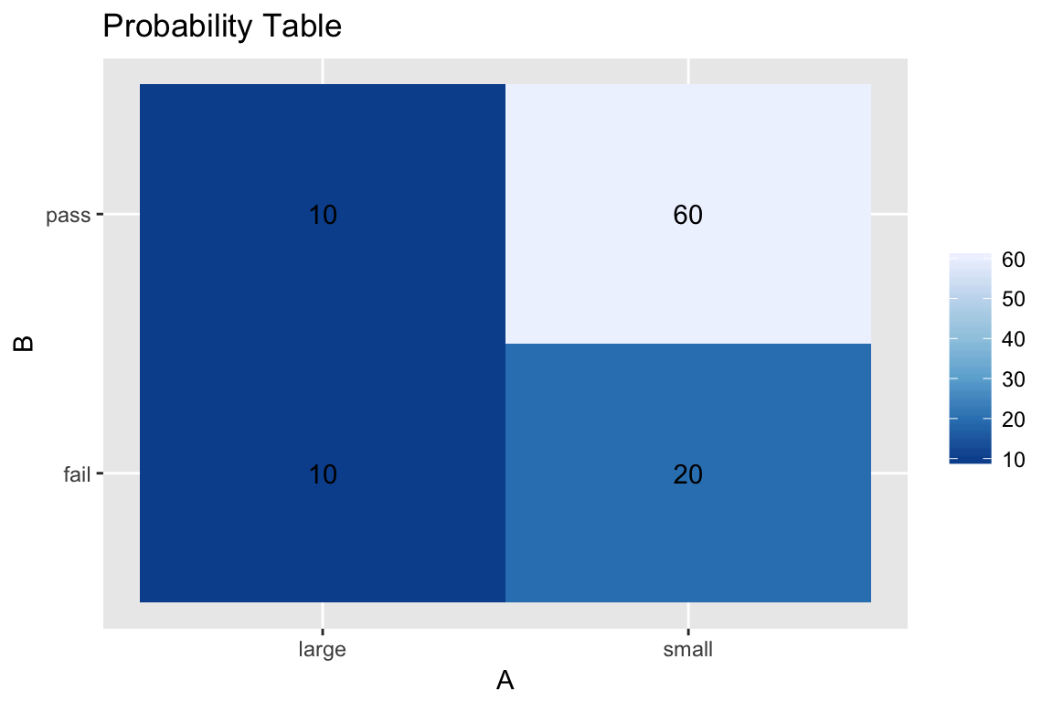
Since we stated this directly earlier, we know that \(p(A=S)=0.8\) and \(p(A=L) = 0.2\) (where \(L\) and \(S\) stand for large and small cities). These are the unconditional, or marginal, probabilities of \(A\) – we don’t care about the air pollution which is event \(B\).
The other information conditional information, e.g. we are told that if \(A=S\), then 60 of 80 pass the test: i.e., \(p(B=P|A=S) = 60/80\) where \(B=P\) indicates a pass and \(B=F\) indicates a failure. Hence, \(p(B=F|A=S)=20/60=0.75\). Similarly, \(p(B=P|A=L)=10/20\) and \(p(B=F|A=L)=0.5\). These are the conditional probabilities, i.e. we make statements about \(B\) given that we know which condition \(A\) is in.
Now, let us see if we can estimate the unconditional probability distribution for \(B\), i.e. the probability that ANY city meets or fails the standard without regard to the size of the city. \[p(B=M) = \frac{(60+10)}{(60+10+20+10)} =0.7\] and \[p(B=F) = \frac{(20+10)}{(60+10+20+10)} =0.3\] which is just the percent of cities that fall in each category.
Now what is left is the definition of the “joint” probability distribution \(p(A,B)\), and the application of Bayes Rule. The joint probability is the chance of a specific condition in both variables. For instance, say we wanted to know the chance of finding a small city that also met the particulate standard, \(p(A=S,B=M) = 60/100\) since there are 60 such cities out of a 100. \(p(A=L,B=F)=10/100\).
Now if we apply Bayes Rule: \[p(A=L |B=M) = \frac{p(A=L,B=M)}{p(B=M)} = 0.1/0.7 = 1/7\] and similarly, \[p(B=M | A=L) = \frac{p(A=L,B=M)}{p(A=L)} =0.1/0.2 =0.5\]
The last statement says that 10% of the cities are large and meet the standard. Since 20% of all the cities are large, then 50% of large cities meet the standard. The conditional statements imply dependence on knowledge of the conditioning variable (the one after the \(|\) line or below the denominator in Bayes Rule).
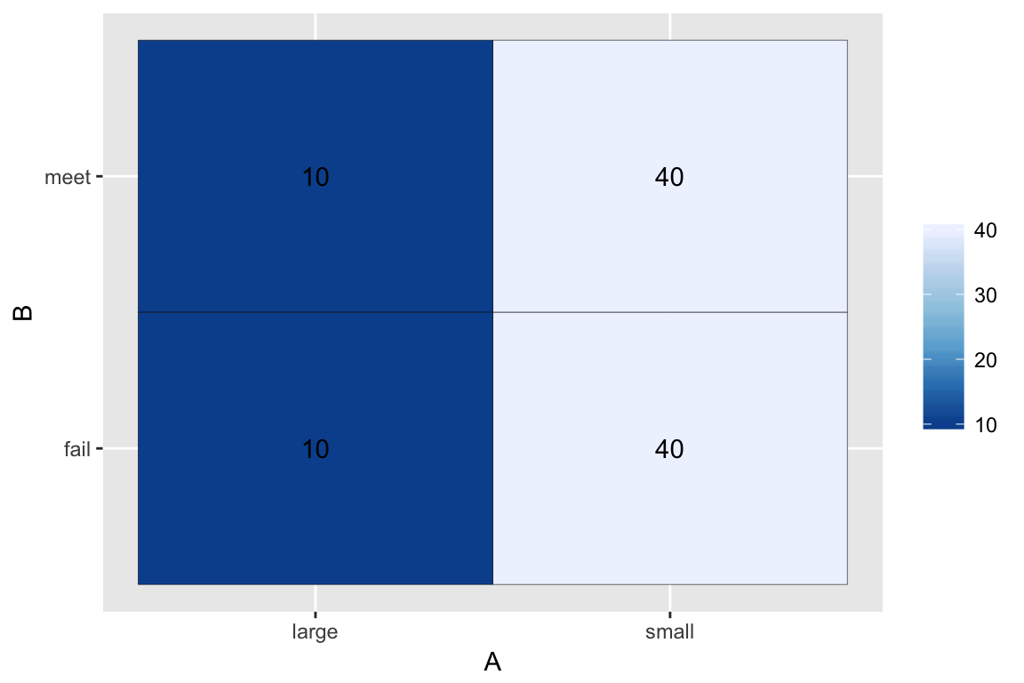
Here’s the new data:
bayes_df <- tibble(A = c('small', 'small', 'large', 'large'),
                   B = c('meet', 'fail', 'meet', 'fail'),
                   count=c(40, 40, 10, 10))
bayes_df %>%
  ggplot(aes(x=A, y=B)) +
  geom_tile(aes(fill=count), color='black') +
  geom_text(aes(label=count), color='black') +
  scale_fill_distiller(palette='Blues', name="")