Chapter 3 Univariate and Multivariate Distributions
A probability distribution records the chance for an outcome (discrete) or the probability density (relative local likelihood in a small interval about the value of interest for a continuous variable). Typically, some distribution functions (equations) are assumed based on past experience or theory. The selection can be based on the admissible domain of the data, e.g. all real values or only positive value, or only values in a certain range.
Exercise 3.1 Check some typical distributions (Normal, Log Normal, Beta, Poisson, Binomial) and identify the key attributes that differ.
Remember that the density or distribution function prescribes the law of probability for that data – i.e. the probabilities corresponding to the population. Given a sample of data, we need to “infer” the best distribution to use, and its parameters. The probability distribution can also be inferred “nonparametrically”. In this case, we don’t assume an underlying functional form for the probability density, but try to approximate any underlying form using a simple procedure – we will study this later on.
Exercise 3.2 In the previous section, last table, which ones are univariate and which ones are bivariate distributions? What kind are they?
Consider formally choosing the best distribution and estimating its parameters. Typically, you choose its parameters by the “best method”, and then see if it is a good fit for the data at hand. There are several criteria for “best” – these include the method of moments, the method of least squares/least absolute deviation and the method of maximum likelihood.
3.1 Moments
For the method of moments the only conceptual idea is that you are trying to match the sample mean, standard deviation etc to the same parameters for the theoretical curve of distribution you have chosen. This is curve matching on the basis of some primary measures of location (mean or median), dispersion (standard deviation or Inter-Quartile range), shape/asymmetry (skew) etc. We will look at this in some more detail later in the semester.
3.2 Likelihood Functions
The sample likelihood is defined as the chance of collectively seeing the set of values that have been observed, given the statistical distribution chosen. If each value \(x_i\) was sampled independently, then the joint probability or likelihood of seeing them collectively is \[\begin{equation} L (x_1, x_2, \ldots, x_n | \theta) = \prod_{i=1}^n f(x_i | \theta) \tag{3.1} \end{equation}\] where \(x_1, x_2, \ldots, x_i, \ldots, x_n\) are different observations, \(\theta\) is the set of parameters of the probability distribution function (for a normal distribution the mean and standard deviation), and \(f(x_i | \theta)\) is the probability density function computed at the particular value \(x_i\) using the parameter value \(\theta\).
3.3 Example
Let us consider the coin toss example and say that the sample we have recorded is H T T T T after 5 tosses of the coin.
Based on this, with no prior information about the coin we would say that \(p(x=H) = 1/5\).
Let us define \(\theta = p(x=H)\) as and consider its estimation using the Likelihood idea.
We’ll vary \(\theta\) over a range of values and compute the likelihood of seeing this sample – here we use the binomial distribution using the dbinom function:
theta <- seq(0, 1, length.out=250)
likelihood <- dbinom(x = 1, size = 5, prob=theta)
plot(theta, likelihood, type='l', main = 'Likelihood of 1 H and 4 T')
abline(v=0.2, col='red', lty='dashed', lwd=3)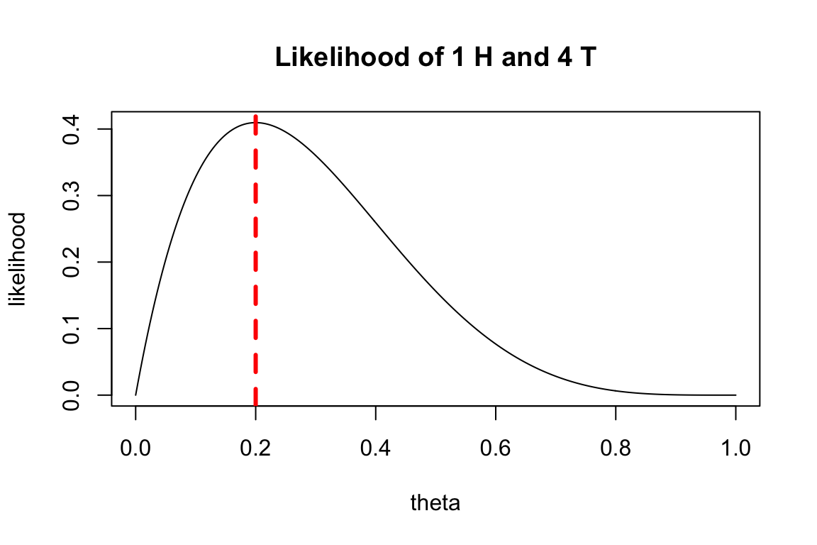
Looking at this, we can see that the most likely – maximum of the likelihood – function is at \(\theta = 0.2\), which is what we previously estimated. However, it’s still possible that we could have gotten these results if \(\theta\) has some other value – near 0.2 is most likely, but we have limited information.
What happens if we had more data: 100 heads out of 500 draws?
likelihood <- dbinom(x = 100, size = 500, prob=theta)
plot(theta, likelihood, type='l', main = 'Likelihood of 100 H and 400 T')
abline(v=0.2, col='red', lty='dashed', lwd=3)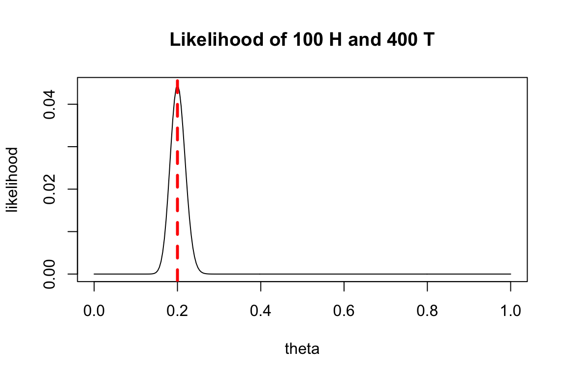
While it’s not implausible that we could get 1 head out of 5 draws if the underlying probability is 0.025 or 0.06, it would be very unlikely for us to get 100 heads out of 500 draws in that case.