2 Imputation of values below LOD
As we can see in the example data (Figure 1.1) some compounds have many low values. These are values below the limit of detection.
2.1 Detection limits
The limit of detection (LOD) is the lowest concentration of an analyte that can be distinguished with reasonable confidence from background noise. The limit of quantification (LOQ) is a value under which the concentration is considered too unreliable to report (Guo, Harel, and Little 2010). For such samples no one concentration can be reported, all that is known is that they are between 0 and LOD or between LOD and LOQ. These are called censored data.
Methods on how to treat censored data in different situations and for different purposes are described at length in Statistics for censored environmental data using Minitab® and R (Helsel 2012). In this document we focus on preparing data to be included as model covariates (and not model outcomes).
Depending on the lab, information on data relative to detection limits is reported differently. Values below LOD can be recorded as: machine readings, “ND”, “.”, etc. These values need special treatment before using them in statistical models. Machine readings are misleading as they are actually just a measure of noise between two values (0 and LOD or LOD and LOQ) that can bias model estimations and diminish statistical power (to be confirmed, need ref). Indicators such as “ND” or “below LOD” cannot be used along with other numeric values in statistical models.
Values between LOD and LOQ usually reported as machine readings should be treated with equal care for the same reasons.
2.2 Imputation below LOD
To be included as covariates in a multivariate model, all data points need a value, including those below the different measurement limits1. For that reason values below LOD or between LOD and LOQ are imputed. There are two families of imputation:
- single imputation: each censored value is replaced by one value
- multiple imputation: each censored value is replaced by a one value but multiple times
Single imputation is simpler, especially when dealing with advanced regression models, but does not account for the variability of the imputation process which artificially reduces the variance (and hence confidence intervals and p-vals) (Lubin et al. 2004).
2.2.1 Single imputation: \(LOD/\sqrt{2}\)
Oftenwise data is simply imputed as \(LOD/\sqrt{2}\). However, simulations show that this method results in substantial bias unless the proportion of missing data is small, ≤ 10% (Lubin et al. 2004).
2.2.2 Single imputation: the fill-in method
A second more elaborate single imputation method consists of randomly drawing values below the LOD (and between LOD and LOQ) from the estimated distribution of the compound. This method is presented in (Helsel 1990) and is referred to as the fill-in method. This method requires a first step of characterising the form of the distribution and estimating its parameters. Censored distribution parameter estimation is described in (Helsel 2012).
The use of a single imputation to fill in missing data using the fill-in method is unbiased or minimally biased quite generally but suffers from inaccurate estimates of variance and, consequently, CIs that are too narrow, particularly, simulations show, when missing data exceed about 30% (Lubin et al. 2004).
Interestingly, with appropriate estimation techniques, this approach accommodates multiple limits, so can be used for imputing values below LOD and also between LOD and LOQ.
Single imputation is sufficient when less of 30% data is censored, and fill-in should systematically be preferred to substitution by \(LOD/\sqrt{2}\).
2.3 Categorisation
For data with more than 30% censored data, values can be multiply imputed2 or categorised as detected/undetected. For the phenols data, data with more than 30% censors was categorised.
2.4 The fill in method in R
The fill-in method consists of 3 steps:
- Log transforming the data as it is a parametric method3
- Computing distributional parameters for the censored data with
NADA::cenros - Replacing the censored data by a random draw from the distribution computed in step 2 and forced to be between -Inf and log(LOD) or between log(LOD) and log(LOQ) with
msm::rtnorm
2.5 Application to the phenols data
The first step is to quantify the amount of data below the different detection limits.
| % below LOD | % below LOQ | |
|---|---|---|
| BPA | 1% | 1% |
| BPAF | 100% | 100% |
| BPB | 100% | 100% |
| BPF | 99% | 99% |
| BPS | 73% | 78% |
| BUPA | 76% | 89% |
| ETPA | 0% | 1% |
| MEPA | 0% | 0% |
| OXBE | 0% | 0% |
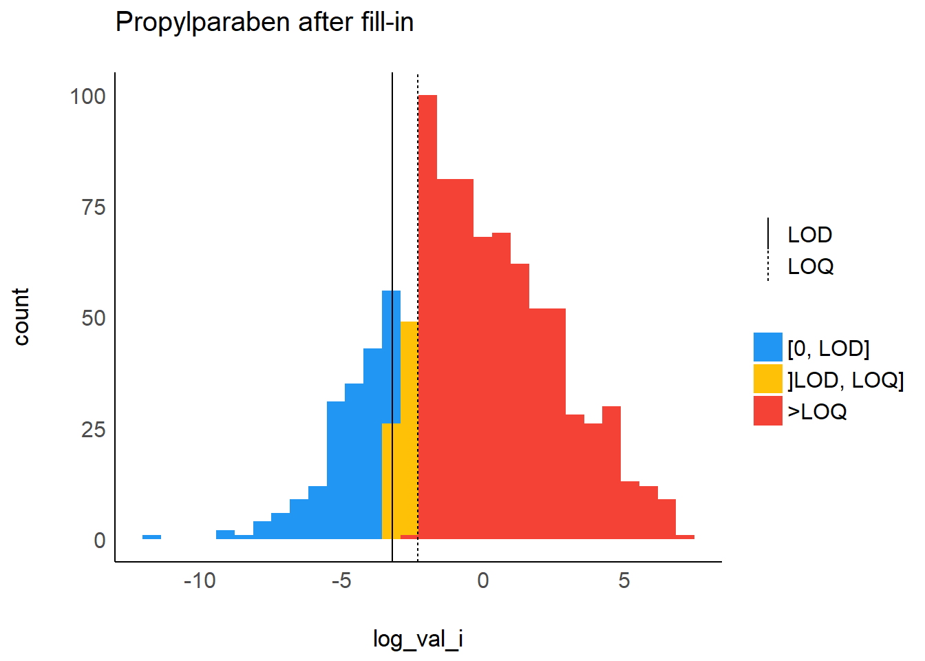
| PRPA | 19% | 27% |
| TRCB | 99% | 100% |
| TRCS | 2% | 2% |
Compounds with more than 95% below LOD are dropped from further analysis:
- BPAF
- BPB
- BPF
- TRCB
According to compound detection rates in Table 2.1, the compounds to categorise are:
- BPS
- BUPA
No further processing takes place on compounds once they are categorised.
The compounds to fill-in are:
- BPA
- ETPA
- MEPA
- OXBE
- PRPA
- TRCS
Example of a filled in compound, PRPA:
This is not true when censored data are to be used as outcomes. In this case data below LOD and between LOD and LOQ can be considered interval censored (Helsel 2012) and analysed with interval regression models such as R’s
survival::survreg[ref papier phenols]. For these models data does not need to be imputed, this is not the topic of this document↩Only valid for 30-50% censored data (Lubin et al. 2004)↩
Although the log transformation does not perform as well as the box-cox transformation, we use the log as it is more robust than the box-cox. Indeed, when applying box-cox, we noticed that correction for protocol variable described in the next chapter was more sensitive to strong corrections producing aberrant values like 2g of MEPA/l of urine.↩