3 Protocol variables
The second main step in our data pre-processing is to correct for protocol variables. Protocol variables are parameters that may influence compound level between sample collection and final concentration The most common example is the measurement batch. The correction method we use is described in (Mortamais et al. 2012) where a multiple linear regression4 is performed for each compound, between the compound level, the protocol variables and adjusted for confounders. And then the relevant model \(\beta\)s are substracted from the measured concentration
The different steps are hence:
- Identify the protocol variables that might have an influence on the compound level
- Identify confounders
- Decide on which protocol variables to actually correct
- Apply correction
3.1 Identification of protocol variables
Variables that we identified in our example data:
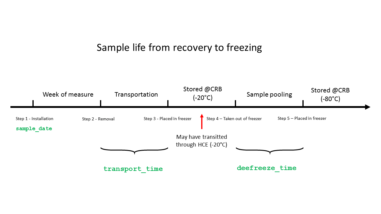
- Time of transport from place of collection to storage freezer (
transport_time) - Defreeze time before sample pooling (
defreeze_time) - Measurement batch when measured at NIPH (
batch)
3.2 Confounders
Using a DAG (not shown here) and the results shown in [phenols paper] we identified the following confounders between phenol level and protocol variables listed previously:
- Specific gravity
- Sample date (linear time trend)
- Sample season (categorical)
- Sampling pregnancy trimester (T1 vs T3)
- Maternal education level (categorical)
- Maternal age (continuous)
- Maternal pre-pregnancy BMI (continuous)
- Parity (continuous)
3.3 Selection of influent variables
Now for each compound we apply the following regression:
\[phenol = protocol\_variables + confounders\]
From this regression we extract Wald’s p to quantify the overall effect of the protocol variable. We will correct for all protocol variables where p < 0.2.
| batch | defreeze_time | transport_time | |
|---|---|---|---|
| BPA | 0 | 0.36 | 0.68 |
| ETPA | 0.06 | 0.93 | 0.29 |
| MEPA | 0.1 | 0.95 | 0.01 |
| MMCHP | 0 | 0.54 | 0.48 |
| OXBE | 0.06 | 0.12 | 0.73 |
| PRPA | 0.02 | 0.73 | 0.08 |
| TRCS | 0.42 | 0.41 | 0.9 |
3.4 Variable correction
Once the protocol variables to correct for are identified for each phenol (in red in Table 3.1) correction on the final values are applied using the (Mortamais et al. 2012) method where:
\[val\_cor_i = val\_crude_i - \sum_i\beta_{protocol\_var\ j} * (X_j^i - X_j^{ref})\] Where:
- \(i\) represents the ith individual
- \(j\) represents the jth protocol variable
- \(X_j^i\) the value of the jth protocol variable for the ith individual
- \(X_j^{ref}\) the chosen reference for protocol variable j (median for continuous variables and highest N category for categorical)
Example:
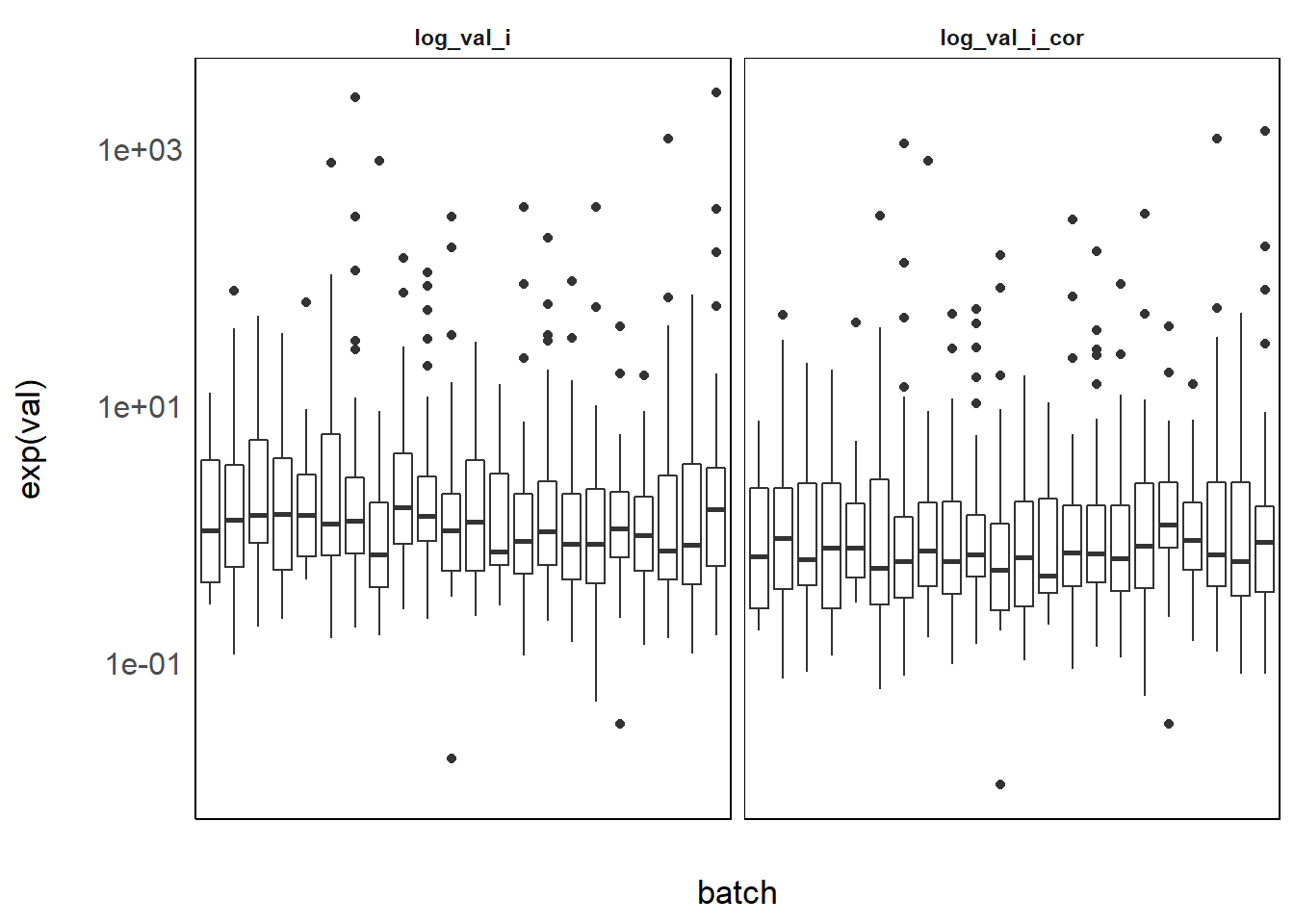
Figure 3.1: Benzophenone-3 levels per batch before and after correction
There still is strong residual variability between batches because phenols are known to vary a lot with season [papier phenols] and season varies strongly accross batch. Here is another example on MMCHP, a phthalate for which we used the same method:
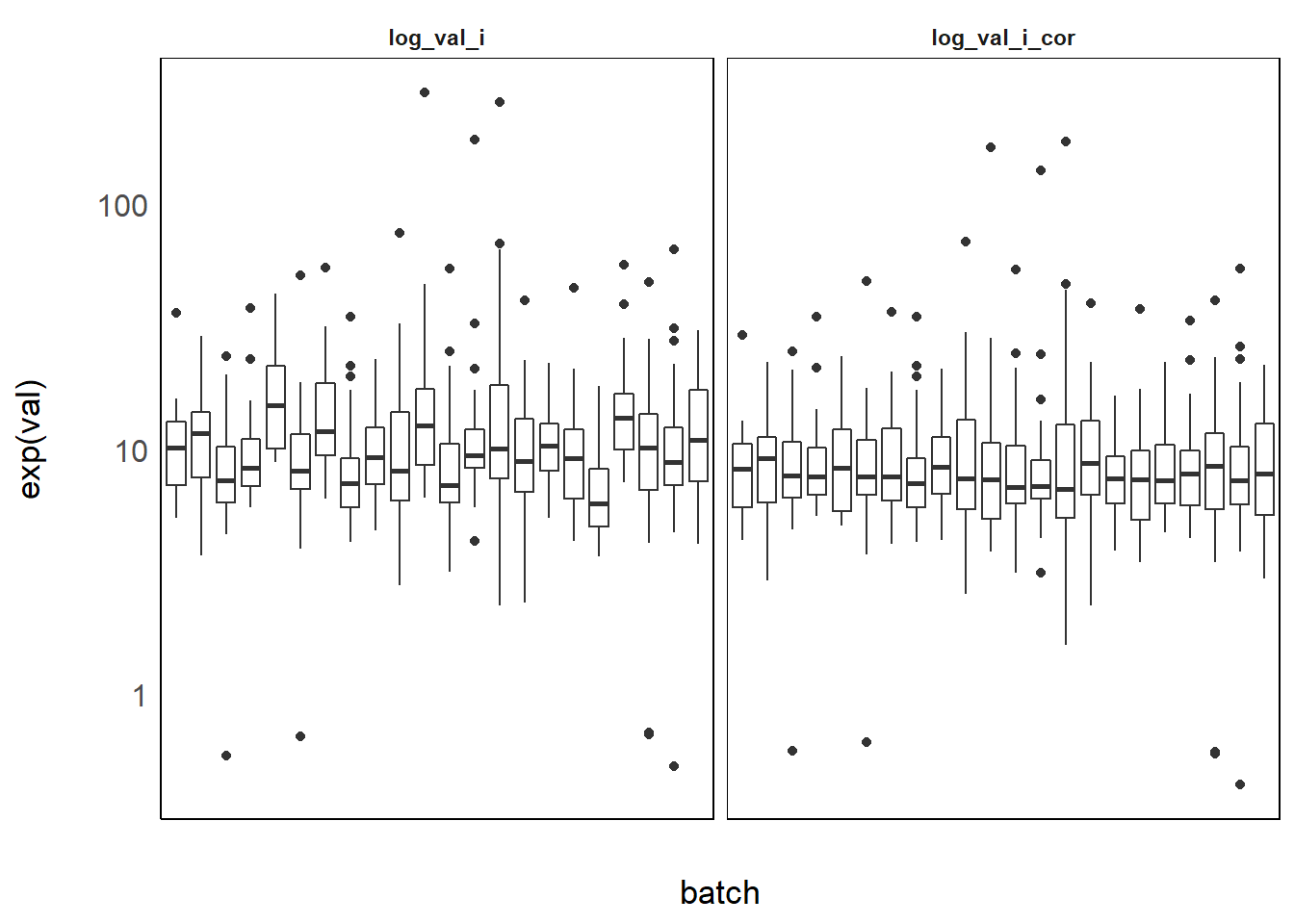
Figure 3.2: MMCHP levels per batch before and after correction
Given that here phenol is the outcome, an interval censored regression such as R’s
survival::survregcould be used where values below LOD are considered censored between 0 and LOD↩