This chapter will provide a gentle introduction to reactive programming, teaching you the basics of the most common reactive constructs you’ll use in Shiny apps.
The input argument is a list-like object that contains all the input data sent from the browser, named according to the input ID. Unlike a typical list, input objects are read-only. If you attempt to modify an input inside the server function, you’ll get an error.
The error occurs because input reflects what’s happening in the browser, and the browser is Shiny’s “single source of truth”. If you could modify the value in R, you could introduce inconsistencies, where the input slider said one thing in the browser, and input$count said something different in R. That would make programming challenging! (Later, in Chapter 8, you’ll learn how to use functions like shiny::updateNumericInput() to modify the value in the browser, and then input$count will update accordingly.)
One more important thing about input: it’s selective about who is allowed to read it. To read from an input, you must be in a reactive context created by a function like shiny::renderText() or shiny::reactive().
3.2.2 Output
output is very similar to input: it’s also a list-like object named according to the output ID. The main difference is that you use it for sending output instead of receiving input. You always use the output object in concert with a render function.
The render function does two things:
It sets up a special reactive context that automatically tracks what inputs the output uses.
It converts the output of your R code into HTML suitable for display on a web page.
Like the input, the output is picky about how you use it. You’ll get an error if:
You forget the render function.
You attempt to read from an output.
3.3 Reactive programming
An app is going to be pretty boring if it only has inputs or only has outputs. The real magic of Shiny happens when you have an app with both.
R Code 3.1 : Interactive greeting as an example for reactive programming
Listing / Output 3.1
Code
ui<-shiny::fluidPage(shiny::textInput("name", "What's your name?"),shiny::textOutput("greeting"))server<-function(input, output, session){output$greeting<-shiny::renderText({paste0("Hello ", input$name, "!")})}shiny::shinyApp(ui, server)
#| '!! shinylive warning !!': |
#| shinylive does not work in self-contained HTML documents.
#| Please set `embed-resources: false` in your metadata.
#| standalone: true
ui <- shiny::fluidPage(
  shiny::textInput("name", "What's your name?"),
  shiny::textOutput("greeting")
)

server <- function(input, output, session) {
  output$greeting <- shiny::renderText({
    paste0("Hello ", input$name, "!")
  })
}

shiny::shinyApp(ui, server)
This is the big idea in Shiny: you don’t need to tell an output when to update, because Shiny automatically figures it out for you.
Important
It’s Shiny’s responsibility to decide when code is executed, not yours. Think of your app as providing Shiny with recipes, not giving it commands.
3.3.1 Imperative vs declarative programming
This difference between commands and recipes is one of the key differences between two important styles of programming:
In imperative programming, you issue a specific command and it’s carried out immediately. This is the style of programming you’re used to in your analysis scripts: you command R to load your data, transform it, visualise it, and save the results to disk.
In declarative programming, you express higher-level goals or describe important constraints, and rely on someone else to decide how and/or when to translate that into action. This is the style of programming you use in Shiny.
With imperative code you say “Make me a sandwich”. With declarative code you say “Ensure there is a sandwich in the refrigerator whenever I look inside of it”. Imperative code is assertive; declarative code is passive-aggressive.
3.3.2 Lazyness
One of the strengths of declarative programming in Shiny is that it allows apps to be extremely lazy. A Shiny app will only ever do the minimal amount of work needed to update the output controls that you can currently see. This laziness, however, comes with an important downside that you should be aware of.
Important
If you’re working on a Shiny app and you just can’t figure out why your code never gets run, double check that your UI and server functions are using the same identifiers.
3.3.3 The reactive graph
Shiny’s laziness has another important property. In most R code, you can understand the order of execution by reading the code from top to bottom. That doesn’t work in Shiny, because code is only run when needed. To understand the order of execution you need to instead look at the reactive graph, which describes how inputs and outputs are connected.
Picture 3.1: This is the reactive graph for R Code 3.3. It shows how the inputs and outputs are connected
The reactive graph contains one symbol for every input and output, and we connect an input to an output whenever the output accesses the input. This graph tells you that greeting will need to be recomputed whenever name is changed. We’ll often describe this relationship as greeting has a reactive dependency on name.
Note the graphical conventions we used for the inputs and outputs: the name input naturally fits into the greeting output.
Picture 3.2: The shapes used by the components of the reactive graph evoke the ways in which they connect.
The reactive graph is a powerful tool for understanding how your app works. As your app gets more complicated, it’s often useful to make a quick high-level sketch of the reactive graph to remind you how all the pieces fit together. Throughout this book we’ll show you the reactive graph to help understand how the examples work, and later on, in Chapter 14, you’ll learn how to use {reactlog} which will draw the graph for you.
3.3.4 Reactive expressions
There’s one more important component that you’ll see in the reactive graph: the reactive expression. We’ll come back to reactive expressions in detail very shortly; for now think of them as a tool that reduces duplication in your reactive code by introducing additional nodes into the reactive graph.
We don’t need a reactive expression in our very simple app, but I’ll add one anyway so you can see how it affects the reactive graph (see Picture 3.3).
R Code 3.2 : Interactive greeting as an example for reactive programming
Listing / Output 3.2
Code
ui<-shiny::fluidPage(shiny::textInput("name", "What's your name?"),shiny::textOutput("greeting"))server<-function(input, output, session){output$greeting<-shiny::renderText(string())string<-shiny::reactive(paste0("Hello ", input$name, "!"))}shiny::shinyApp(ui, server)
#| '!! shinylive warning !!': |
#| shinylive does not work in self-contained HTML documents.
#| Please set `embed-resources: false` in your metadata.
#| standalone: true
ui <- shiny::fluidPage(
shiny::textInput("name", "What's your name?"),
shiny::textOutput("greeting")
)
server <- function(input, output, session) {
string <- shiny::reactive(paste0("Hello ", input$name, "!"))
output$greeting <- shiny::renderText(string())
}
shiny::shinyApp(ui, server)
Picture 3.3: A reactive expression is drawn with angles on both sides because it connects inputs to outputs.
Reactive expressions take inputs and produce outputs so they have a shape that combines features of both inputs and outputs.
3.3.5 Execution order
It’s important to understand that the order in which your code runs is solely determined by the reactive graph. This is different from most R code where the execution order is determined by the order of lines. For example, we could flip the order of the two lines in our simple server function:
R Code 3.3 : Interactive greeting as an example for reactive programming
Listing / Output 3.3
Code
ui<-shiny::fluidPage(shiny::textInput("name", "What's your name?"),shiny::textOutput("greeting"))server<-function(input, output, session){string<-shiny::reactive(paste0("Hello ", input$name, "!"))output$greeting<-shiny::renderText(string())}shiny::shinyApp(ui, server)
#| '!! shinylive warning !!': |
#| shinylive does not work in self-contained HTML documents.
#| Please set `embed-resources: false` in your metadata.
#| standalone: true
ui <- shiny::fluidPage(
  shiny::textInput("name", "What's your name?"),
  shiny::textOutput("greeting")
)

server <- function(input, output, session) {
  output$greeting <- shiny::renderText(string())
  string <- shiny::reactive(paste0("Hello ", input$name, "!"))
}

shiny::shinyApp(ui, server)
Again: Compare the tiny difference in the server code; this time with Listing / Output 3.2.
You might think that this would yield an error because output$greeting refers to a reactive expression, string, that hasn’t been created yet. But remember Shiny is lazy, so that code is only run when the session starts, after string has been created.
Instead, this code yields the same reactive graph as above, so the order in which the code is run is exactly the same. Organizing your code like this is confusing for humans, and best avoided. Instead, make sure that reactive expressions and outputs only refer to things defined above, not below. This will make your code easier to understand.
This concept is very important and different to most other R code, so I’ll say it again:
Important
The order in which reactive code is run is determined only by the reactive graph, not by its layout in the server function.
3.3.6 Exercises
3.3.6.1 Find bugs
Exercise 3.1 : Find the bugs in the three server functions
R Code 3.4 : Find the bugs in the three server functions
Fix the simple errors found in each of the three server functions below. First try spotting the problem just by reading the code; then run the code to make sure you’ve fixed it.
The first two examples of my trials coincide with Mastering Shiny Solutions. In the third example I had a chain of the inputs a,b,c,d and not — as in Mastering Shiny Solutions — a step by step chain where each input is depending of an input with the same name.
Picture 3.4: Solution of the reactive graph: server 1
Picture 3.5: Solution of the reactive graph: server 2
Picture 3.6: Solution of the reactive graph: server 3
In the following solution code from Mastering Shiny Solutions I have followed their idea to change range into col_range and var into col_var. These new names substitute the bad names for the reactives in the failed code snippet.
Compare the Shiny result with the code used for the solution in Listing / Output 3.7.
3.4 Reactive expressions
Reactive expressions have a flavor of both inputs and outputs:
Like outputs, reactive expressions depend on inputs and automatically know when they need updating.
Like inputs, you can use the results of a reactive expression in an output.
This duality means we need some new vocab: I’ll use producers to refer to reactive inputs and expressions, and consumers to refer to reactive expressions and outputs.
Picture 3.7: Inputs and expressions are reactive producers; expressions and outputs are reactive consumers
3.4.1 The motivation
Imagine I want to compare two simulated datasets with a plot and a hypothesis test. I’ve done a little experimentation and come up with the functions below: freqpoly() visualizes the two distributions with frequency polygons, and t_test() uses a t-test to compare means and summarizes the results with a string:
R Code 3.10 : Compare two simulated datasets with a plot and a hypothesis test.
Code
freqpoly<-function(x1, x2, binwidth=0.1, xlim=c(-3, 3)){df<-base::data.frame( x =base::c(x1, x2), g =base::c(base::rep("x1", base::length(x1)), base::rep("x2", base::length(x2))))ggplot2::ggplot(df, ggplot2::aes(x, colour =g))+ggplot2::geom_freqpoly(binwidth =binwidth, linewidth =1)+ggplot2::coord_cartesian(xlim =xlim)}t_test<-function(x1, x2){test<-stats::t.test(x1, x2)# use sprintf() to format t.test() results compactlybase::sprintf("p value: %0.3f\n[%0.2f, %0.2f]",test$p.value, test$conf.int[1], test$conf.int[2])}### prepare valuesx1<-stats::rnorm(100, mean =0, sd =0.5)x2<-stats::rnorm(200, mean =0.15, sd =0.9)### call functionsfreqpoly(x1, x2)base::cat(t_test(x1, x2))
#> p value: 0.001
#> [-0.47, -0.13]
Picture 3.8: Compare two simulated datasets with a plot and a hypothesis test
3.4.2 The app
I’d like to use these two tools to quickly explore a bunch of simulations. A Shiny app is a great way to do this because it lets you avoid tediously modifying and re-running R code. Below I wrap the pieces into a Shiny app where I can interactively tweak the inputs.
Code Collection 3.1 : Case study: Compare simulated data V1
R Code 3.11 : Case study: Compare simulated data V1
Listing / Output 3.8: Compare simulated data with plot and t-test
Code
## source .R file with the two functions didn't work## so I had to use the original code instead of the followingbase::source(base::paste0(here::here(), "/R/shiny-03-V2.R"), local =TRUE, chdir =TRUE, encoding ="utf-8")library(shiny)library(ggplot2)library(munsell)ui<-fluidPage(fluidRow(column(4,"Distribution 1",numericInput("n1", label ="n", value =1000, min =1),numericInput("mean1", label ="µ", value =0, step =0.1),numericInput("sd1", label ="σ", value =0.5, min =0.1, step =0.1)),column(4,"Distribution 2",numericInput("n2", label ="n", value =1000, min =1),numericInput("mean2", label ="µ", value =0, step =0.1),numericInput("sd2", label ="σ", value =0.5, min =0.1, step =0.1)),column(4,"Frequency polygon",numericInput("binwidth", label ="Bin width", value =0.1, step =0.1),sliderInput("range", label ="range", value =c(-3, 3), min =-5, max =5))),fluidRow(column(9, plotOutput("hist")),column(3, verbatimTextOutput("ttest"))))server<-function(input, output, session){output$hist<-renderPlot({x1<-rnorm(input$n1, input$mean1, input$sd1)x2<-rnorm(input$n2, input$mean2, input$sd2)freqpoly(x1, x2, binwidth =input$binwidth, xlim =input$range)}, res =96)output$ttest<-renderText({x1<-rnorm(input$n1, input$mean1, input$sd1)x2<-rnorm(input$n2, input$mean2, input$sd2)t_test(x1, x2)})}shinyApp(ui, server)
R Code 3.12 : Case study: Compare simulated data V1
I had to duplicate the code for the two functions freqpoly() and t_test() because sourcing the code from an extra .R file did not work. I tried several options of source("path-to-file", local = TRUE)
file in an extra directory with additional option chdir = TRUE,
file in main directory references with source('./<file_name>', local=TRUE)
file calling with here::here() applying if(FALSE){library(here)} to include additional R packages that are not automatically discovered,
adding encoding="utf-8"
You can find a live version at https://hadley.shinyapps.io/ms-case-study-1; I recommend opening the app with the above link, because it uses the whole screen width and it is therefore easier to play with. Having a quick play to make sure you understand its basic operation is essential before you continue reading.
3.4.3 The reactive graph
Shiny is smart enough to update an output only when the inputs it refers to change; it’s not smart enough to only selectively run pieces of code inside an output. In other words, outputs are atomic: they’re either executed or not as a whole.
As a human reading this code you can tell that we only need to update x1 when n1, mean1, or sd1 changes, and we only need to update x2 when n2, mean2, or sd2 changes. Shiny, however, only looks at the output as a whole, so it will update both x1 and x2 every time one of n1, mean1, sd1, n2, mean2, or sd2 changes. This leads to the reactive graph shown in Picture 3.9.
Picture 3.9: The reactive graph shows that every output depends on every input
You’ll notice that the graph is very dense: almost every input is connected directly to every output. This creates two problems:
The app is hard to understand because there are so many connections. There are no pieces of the app that you can pull out and analyse in isolation.
The app is inefficient because it does more work than necessary. For example, if you change the breaks of the plot, the data is recalculated; if you change the value of n1, x2 is updated (in two places!).
There’s one other major flaw in the app: the frequency polygon and t-test use separate random draws. This is rather misleading, as you’d expect them to be working on the same underlying data.
Fortunately, we can fix all these problems by using reactive expressions to pull out repeated computation.
3.4.4 Simplifying the graph
Code Collection 3.2 : Case study: Compare simulated data V2
R Code 3.13 : Case study: Compare simulated data V2
Listing / Output 3.9: Compare simulated data with plot and t-test using reactive expressions
Code
## source .R file with the two functions didn't workbase::source(base::paste0(here::here(), "/R/shiny-03-V2.R"), local =TRUE, chdir =TRUE, encoding ="utf-8")library(shiny)library(ggplot2)library(munsell)ui<-fluidPage(fluidRow(column(4,"Distribution 1",numericInput("n1", label ="n", value =1000, min =1),numericInput("mean1", label ="µ", value =0, step =0.1),numericInput("sd1", label ="σ", value =0.5, min =0.1, step =0.1)),column(4,"Distribution 2",numericInput("n2", label ="n", value =1000, min =1),numericInput("mean2", label ="µ", value =0, step =0.1),numericInput("sd2", label ="σ", value =0.5, min =0.1, step =0.1)),column(4,"Frequency polygon",numericInput("binwidth", label ="Bin width", value =0.1, step =0.1),sliderInput("range", label ="range", value =c(-3, 3), min =-5, max =5))),fluidRow(column(9, plotOutput("hist")),column(3, verbatimTextOutput("ttest"))))server<-function(input, output, session){x1<-reactive(rnorm(input$n1, input$mean1, input$sd1))x2<-reactive(rnorm(input$n2, input$mean2, input$sd2))output$hist<-renderPlot({freqpoly(x1(), x2(), binwidth =input$binwidth, xlim =input$range)}, res =96)output$ttest<-renderText({t_test(x1(), x2())})}shinyApp(ui, server)
Compare the code in Listing / Output 3.8 for this shiny app without reactive expressions
R Code 3.14 : Case study: Compare simulated data V2
#| '!! shinylive warning !!': |
#|   shinylive does not work in self-contained HTML documents.
#|   Please set `embed-resources: false` in your metadata.
#| standalone: true
#| viewerHeight: 600


# source .R file with the two functions didn't work
freqpoly <- function(x1, x2, binwidth = 0.1, xlim = c(-3, 3)) {
    df <- base::data.frame(
        x = base::c(x1, x2),
        g = base::c(base::rep("x1", base::length(x1)),
                    base::rep("x2", base::length(x2)))
    )

    ggplot2::ggplot(df, ggplot2::aes(x, colour = g)) +
        ggplot2::geom_freqpoly(binwidth = binwidth, linewidth = 1) +
        ggplot2::coord_cartesian(xlim = xlim)
}

t_test <- function(x1, x2) {
    test <- stats::t.test(x1, x2)

    # use sprintf() to format t.test() results compactly
    base::sprintf(
        "p value: %0.3f\n[%0.2f, %0.2f]",
        test$p.value, test$conf.int[1], test$conf.int[2]
    )
}

# base::source(
#       base::paste0(here::here(), "/R/shiny-03-V2.R"),
#       local = TRUE,
#       chdir = TRUE,
#       encoding = "utf-8"
#     )

library(shiny)
library(ggplot2)
library(munsell)

ui <- fluidPage(
  fluidRow(
    column(4,
      "Distribution 1",
      numericInput("n1", label = "n", value = 1000, min = 1),
      numericInput("mean1", label = "µ", value = 0, step = 0.1),
      numericInput("sd1", label = "σ", value = 0.5, min = 0.1, step = 0.1)
    ),
    column(4,
      "Distribution 2",
      numericInput("n2", label = "n", value = 1000, min = 1),
      numericInput("mean2", label = "µ", value = 0, step = 0.1),
      numericInput("sd2", label = "σ", value = 0.5, min = 0.1, step = 0.1)
    ),
    column(4,
      "Frequency polygon",
      numericInput("binwidth", label = "Bin width", value = 0.1, step = 0.1),
      sliderInput("range", label = "range", value = c(-3, 3), min = -5, max = 5)
    )
  ),
  fluidRow(
    column(9, plotOutput("hist")),
    column(3, verbatimTextOutput("ttest"))
  )
)

server <- function(input, output, session) {
  x1 <- reactive(rnorm(input$n1, input$mean1, input$sd1))
  x2 <- reactive(rnorm(input$n2, input$mean2, input$sd2))

  output$hist <- renderPlot({
    freqpoly(x1(), x2(), binwidth = input$binwidth, xlim = input$range)
  }, res = 96)

  output$ttest <- renderText({
    t_test(x1(), x2())
  })
}

shinyApp(ui, server)
This transformation yields the substantially simpler graph shown in Picture 3.10. This simpler graph makes it easier to understand the app because you can understand connected components in isolation; the values of the distribution parameters only affect the output via x1 and x2. This rewrite also makes the app much more efficient since it does much less computation. Now, when you change the binwidth or range, only the plot changes, not the underlying data.
Picture 3.10: Using reactive expressions considerably simplifies the graph, making it much easier to understand
To emphasize this modularity Picture 3.11 draws boxes around the independent components. We’ll come back to this idea in Chapter 19, when we discuss modules. Modules allow you to extract out repeated code for reuse, while guaranteeing that it’s isolated from everything else in the app. Modules are an extremely useful and powerful technique for more complex apps.
Picture 3.11: Modules enforce isolation between parts of an app
You might be familiar with the “rule of three” of programming: whenever you copy and paste something three times, you should figure out how to reduce the duplication (typically by writing a function). In Shiny, however, you should consider the rule of one: whenever you copy and paste something once, you should consider extracting the repeated code out into a reactive expression. The rule is stricter for Shiny because reactive expressions don’t just make it easier for humans to understand the code, they also improve Shiny’s ability to efficiently rerun code.
3.4.5 Why do we need reactive expressions?
When you first start working with reactive code, you might wonder why we need reactive expressions. Why can’t you use your existing tools for reducing duplication in code: creating new variables and writing functions? Unfortunately neither of these techniques work in a reactive environment.
If you try to use a variable to reduce duplication, you’ll get an error because you’re attempting to access input values outside of a reactive context. Even if you didn’t get that error, you’d still have a problem: x1 and x2 would only be computed once, when the session begins, not every time one of the inputs was updated.
If you try to use a function to reduce duplication it has the same problem as the original code: any input will cause all outputs to be recomputed, and the t-test and the frequency polygon will be run on separate samples. Reactive expressions automatically cache their results, and only update when their inputs change.
3.5 Controlling timing of evaluation
Now that you’re familiar with the basic ideas of reactivity, we’ll discuss two more advanced techniques that allow you to either increase or decrease how often a reactive expression is executed. Here I’ll show how to use the basic techniques; in Chapter 15, we’ll come back to their underlying implementations.
To explore the basic ideas, I’m going to simplify my simulation app. I’ll use a distribution with only one parameter, and force both samples to share the same n. I’ll also remove the plot controls. This yields a smaller UI object and server function.
Code Collection 3.3 : Case study: Compare simulated data V3
Compare the code with original app Listing / Output 3.8 (without reactive expression) and Listing / Output 3.9 (with reactive expressions) with this more simpler app that draws from two Poisson distributions.
R Code 3.16 : Case study: Compare simulated data V3
#| '!! shinylive warning !!': |
#|   shinylive does not work in self-contained HTML documents.
#|   Please set `embed-resources: false` in your metadata.
#| standalone: true
#| viewerHeight: 600

# source .R file with the two functions didn't work
freqpoly <- function(x1, x2, binwidth = 0.1, xlim = c(-3, 3)) {
    df <- base::data.frame(
        x = base::c(x1, x2),
        g = base::c(base::rep("x1", base::length(x1)),
                    base::rep("x2", base::length(x2)))
    )

    ggplot2::ggplot(df, ggplot2::aes(x, colour = g)) +
        ggplot2::geom_freqpoly(binwidth = binwidth, linewidth = 1) +
        ggplot2::coord_cartesian(xlim = xlim)
}

t_test <- function(x1, x2) {
    test <- stats::t.test(x1, x2)

    # use sprintf() to format t.test() results compactly
    base::sprintf(
        "p value: %0.3f\n[%0.2f, %0.2f]",
        test$p.value, test$conf.int[1], test$conf.int[2]
    )
}

# base::source(
#       base::paste0(here::here(), "/R/shiny-03-V2.R"),
#       local = TRUE,
#       chdir = TRUE,
#       encoding = "utf-8"
#     )

library(shiny)
library(ggplot2)
library(munsell)

ui <- fluidPage(
  fluidRow(
    column(3,
      numericInput("lambda1", label = "lambda1", value = 3),
      numericInput("lambda2", label = "lambda2", value = 5),
      numericInput("n", label = "n", value = 1e4, min = 0)
    ),
    column(9, plotOutput("hist"))
  )
)
server <- function(input, output, session) {
  x1 <- reactive(rpois(input$n, input$lambda1))
  x2 <- reactive(rpois(input$n, input$lambda2))
  output$hist <- renderPlot({
    freqpoly(x1(), x2(), binwidth = 1, xlim = c(0, 40))
  }, res = 96)
}

shinyApp(ui, server)
Picture 3.12: The reactive graph of a simpler app that displays a frequency polygon of random numbers drawn from two Poisson distributions.
3.5.1 Timed invalidation
Imagine you wanted to reinforce the fact that this is for simulated data by constantly resimulating the data, so that you see an animation rather than a static plot. We can increase the frequency of updates with a new function: shiny::reactiveTimer().
shiny::reactiveTimer() is a reactive expression that has a dependency on a hidden input: the current time. You can use a reactiveTimer() when you want a reactive expression to invalidate itself more often than it otherwise would. For example, the following code uses an interval of 500 ms so that the plot will update twice a second. This is fast enough to remind you that you’re looking at a simulation, without dizzying you with rapid changes.
Code Collection 3.4 : Case study: Compare simulated data V4
Note how we use timer() in the reactive expressions that compute x1() and x2(): we call it, but don’t use the value. This lets x1 and x2 take a reactive dependency on timer, without worrying about exactly what value it returns.
In the above scenario, think about what would happen if the simulation code took 1 second to run. We perform the simulation every 0.5s, so Shiny would have more and more to do, and would never be able to catch up. The same problem can happen if someone is rapidly clicking buttons in your app and the computation you are doing is relatively expensive. It’s possible to create a big backlog of work for Shiny, and while it’s working on the backlog, it can’t respond to any new events. This leads to a poor user experience.
If this situation arises in your app, you might want to require the user to opt-in to performing the expensive calculation by requiring them to click a button. This is a great use case for an shiny::actionButton().
Code Collection 3.5 : Case study: Compare simulated data V5 (action button V1)
R Code 3.20 : Case study: Compare simulated data V5 (action button V1)
#| '!! shinylive warning !!': |
#|   shinylive does not work in self-contained HTML documents.
#|   Please set `embed-resources: false` in your metadata.
#| standalone: true
#| viewerHeight: 600

# source .R file with the two functions didn't work
freqpoly <- function(x1, x2, binwidth = 0.1, xlim = c(-3, 3)) {
    df <- base::data.frame(
        x = base::c(x1, x2),
        g = base::c(base::rep("x1", base::length(x1)),
                    base::rep("x2", base::length(x2)))
    )

    ggplot2::ggplot(df, ggplot2::aes(x, colour = g)) +
        ggplot2::geom_freqpoly(binwidth = binwidth, linewidth = 1) +
        ggplot2::coord_cartesian(xlim = xlim)
}

t_test <- function(x1, x2) {
    test <- stats::t.test(x1, x2)

    # use sprintf() to format t.test() results compactly
    base::sprintf(
        "p value: %0.3f\n[%0.2f, %0.2f]",
        test$p.value, test$conf.int[1], test$conf.int[2]
    )
}

# source(
#       paste0(here::here(), "/R/shiny-03-V2.R"),
#       local = TRUE,
#       chdir = TRUE,
#       encoding = "utf-8"
#     )

library(shiny)
library(ggplot2)
library(munsell)

ui <- fluidPage(
  fluidRow(
    column(3,
      numericInput("lambda1", label = "lambda1", value = 3),
      numericInput("lambda2", label = "lambda2", value = 5),
      numericInput("n", label = "n", value = 1e4, min = 0),
      actionButton("simulate", "Simulate!")
    ),
    column(9, plotOutput("hist"))
  )
)

server <- function(input, output, session) {
  x1 <- reactive({
    input$simulate
    rpois(input$n, input$lambda1)
  })
  x2 <- reactive({
    input$simulate
    rpois(input$n, input$lambda2)
  })
  output$hist <- renderPlot({
    freqpoly(x1(), x2(), binwidth = 1, xlim = c(0, 40))
  }, res = 96)
}

shinyApp(ui, server)
Press the “Simulate” button to compare another step of the two Poison distribution. But observe that changes in the input field also start the calculation and redrawing of the graph. This code doesn’t accomplish our goal; we’ve added another dependency instead of replacing the existing dependencies.
R Code 3.22 : Case study: Compare simulated data V6 (action button V2)
#| '!! shinylive warning !!': |
#|   shinylive does not work in self-contained HTML documents.
#|   Please set `embed-resources: false` in your metadata.
#| standalone: true
#| viewerHeight: 600

# source .R file with the two functions didn't work
freqpoly <- function(x1, x2, binwidth = 0.1, xlim = c(-3, 3)) {
    df <- base::data.frame(
        x = base::c(x1, x2),
        g = base::c(base::rep("x1", base::length(x1)),
                    base::rep("x2", base::length(x2)))
    )

    ggplot2::ggplot(df, ggplot2::aes(x, colour = g)) +
        ggplot2::geom_freqpoly(binwidth = binwidth, linewidth = 1) +
        ggplot2::coord_cartesian(xlim = xlim)
}

t_test <- function(x1, x2) {
    test <- stats::t.test(x1, x2)

    # use sprintf() to format t.test() results compactly
    base::sprintf(
        "p value: %0.3f\n[%0.2f, %0.2f]",
        test$p.value, test$conf.int[1], test$conf.int[2]
    )
}

# source(
#       paste0(here::here(), "/R/shiny-03-V2.R"),
#       local = TRUE,
#       chdir = TRUE,
#       encoding = "utf-8"
#     )

library(shiny)
library(ggplot2)
library(munsell)

ui <- fluidPage(
  fluidRow(
    column(3,
      numericInput("lambda1", label = "lambda1", value = 3),
      numericInput("lambda2", label = "lambda2", value = 5),
      numericInput("n", label = "n", value = 1e4, min = 0),
      actionButton("simulate", "Simulate!")
    ),
    column(9, plotOutput("hist"))
  )
)

server <- function(input, output, session) {
  x1 <- eventReactive(input$simulate, {
    rpois(input$n, input$lambda1)
  })
  x2 <- eventReactive(input$simulate, {
    rpois(input$n, input$lambda2)
  })

  output$hist <- renderPlot({
    freqpoly(x1(), x2(), binwidth = 1, xlim = c(0, 40))
  }, res = 96)
}

shinyApp(ui, server)
Press the “Simulate” button to compare another step of the two Poison distribution. Observe that changes in the input field does not start the calculation and redrawing of the graph.
Picture 3.15: shiny::eventReactive() makes it possible to separate the dependencies (black arrows) from the values used to compute the result (pale gray arrows).
3.6 Observers
So far, we’ve focused on what’s happening inside the app. But sometimes you need to reach outside of the app and cause side-effects to happen elsewhere in the world. This might be saving a file to a shared network drive, sending data to a web API, updating a database, or (most commonly) printing a debugging message to the console. These actions don’t affect how your app looks, so you shouldn’t use an output and a render function. Instead you need to use an observer.
There are multiple ways to create an observer, and we’ll come back to them later in Section 15.3. For now, I wanted to show you how to use shiny::observeEvent(), because it gives you an important debugging tool when you’re first learning Shiny.
shiny::observeEvent() does work as a separate app, but does not work with {shinylive}, e.g. it does not send a message neither to the console nor to the HTML web page. I assume it has again to do with variable scoping rules or with the {shinylive} configuration.
You don’t assign the result of observeEvent() to a variable, so
You can’t refer to it from other reactive consumers.
Observers and outputs are closely related. You can think of outputs as having a special side-effect: updating the HTML in the user’s browser. To emphasize this closeness, we’ll draw them the same way in the reactive graph. This yields the following reactive graph shown in Picture 3.16.
Picture 3.16: In the reactive graph, an observer looks the same as an output
3.7 Summary
Note
This is already my third reading of this chapter. Each reading lies about one year apart.
The first and second time I thought that each example is easy to understand and that the chapter as a whole is straightforward. But it turned out that I was wrong!
As a summary I will I will again read the text. But this time I will pay attention to each line of code and write down every tiny example. Additionally I will create my own example and / or invoke the debugger to experiment with the code to understand exactly what is happening inside the server part.
There is no error if you run this code. But there is no output as well! The result is an empty white pane.
3.7.2 Printing messages from ui and server part
The problem in my understanding became obvious, when I tried to display just one text message inside the ui() and the other one from inside the server() function. To make my difficulties explicit I will separate the task in several steps.
Experiment 3.1 : Printing messages from ui and server part
As you can see only the print statement from the UI is visible. The app does not produce an error and it even produces an output from the server function to the console. But the server print statement does not appear inside the app.
I will now list several approaches that will fail with their error messages. I hope that this would be helpful to understand better the effect of the reactive context.
But I have to fake the error messages as with the shinylive extension Shiny will either only produce an empty white pane or display a different error message. I create therefore external Shiny apps, run them with the wrong code snippets and copy the generated error message in this Quarto document.
Experiment 3.2 : Why several other approaches will fail?
Error in $<-(*tmp*, msg, value = “back end logic”) :
Can’t modify read-only reactive value ‘msg’
The input argument is a list-like object, but unlike a typical list, input objects are read-only. If you attempt to modify an input inside the server function, you’ll get the above error.
Note
This error occurs because input reflects what’s happening in the browser, and the browser is Shiny’s “single source of truth”. If you could modify the value in R, you could introduce inconsistencies, where the input text said one thing in the browser, and input$msg said something different in R. That would make programming challenging! Later, in Chapter 8, you’ll learn how to use functions like updateTextInput() to modify the value in the browser, and then input$msg will update accordingly.
R Code 3.29 : Reading from input needs a reactive context
Listing / Output 3.19: To read from an input, you must be in a reactive context.
Error in input$msg :
Can’t access reactive value ‘msg’ outside of reactive consumer.
ℹ Do you need to wrap inside reactive() or observe()?
input is selective about who is allowed to read it. To read from an input, you must be in a reactive context created by a function like renderText() or reactive(). This is an important constraint that allows outputs to automatically update when an input changes.
R Code 3.30 : output needs a render function
Listing / Output 3.20: output needs a reactive context, it has to be inside a render function.
The important point of reactive expressions is that they mediate between input and output. string works as an mediator between input$name and output$greeting.
We can think of reactive expressions as tools to reduces duplication in the reactive code by introducing additional nodes into the reactive graph. Te reactive expression can be used like a function and like a function it is called with () at the end of its name. But it never has arguments between its parenthesis.
3.7.5.2 Practical example
In the case above we didn’t use the additional node, to simplify the code. In order to understand why we need reactive epxressions we need a more complex example. Hadley offers in the book the comparison of two simulated datasets with a plot and a hypothesis test.
A frequency polygon is a histogram that's drawn with a line, instead of bars, which makes it easier to compare multiple data sets on the same plot.
Observer
In R Shiny, an observer is a function that can read reactive values and call reactive expressions, and it will automatically re-execute when those dependencies change. Unlike reactive expressions, observers do not yield a result and cannot be used as an input to other reactive expressions. Instead, they are useful for their side effects, such as performing I/O operations.
Reactive context
In Shiny, reactive contexts are essential for handling user inputs and updating outputs automatically. Reactive values can only be accessed within a reactive context, meaning they must be used inside functions like `reactive()`, `observer()`, or any `render*()` functions.
Reactive dependencies
In Shiny, reactive dependencies are automatically inferred by the framework, meaning that when you define a reactive expression, Shiny determines which inputs it depends on. For example, if you have a reactive expression `b <- reactive(a * 2)`, Shiny infers that `b` depends on `a`. This information is stored internally within the Shiny framework, but it is not directly accessible through standard functions. For more detailed control over dependencies, you might consider using `isolate()` to prevent certain parts of your code from being reactive, or using `reactiveValues()` to manage stateful objects that can be updated and accessed across different parts of your application.
reactive epxressions
Reactive expressions
Reactive expressions are a key component of reactive programming in Shiny. They are R expressions that use widget input and return a value, updating this value whenever the original widget changes. Reactive expressions cache their values and know when their values have become outdated, which helps in preventing unnecessary re-computation and makes the app faster.
Reactive graph
In Shiny, the reactive graph is a powerful tool for understanding how your app works. It shows how inputs and outputs are connected, allowing you to visualize the dependencies and execution order of your reactive expressions and render functions. This graph is particularly useful as your app becomes more complex, helping you to manage and debug the interdependencies between different components of your app. To visualize the reactive graph, you can use the reactlog package, which provides an interactive browser-based tool for visualizing reactive dependencies and execution in your application.
---execute: cache: true---# Basic reactivity {#sec-chap03}```{r}#| label: setup#| results: hold#| include: falsebase::source(file ="R/helper.R")ggplot2::theme_set(ggplot2::theme_bw())options(show.signif.stars =FALSE)```## Introduction::::: {#obj-chap03}:::: {.my-objectives}::: {.my-objectives-header}Objectives and chapter section list:::::: {.my-objectives-container}This chapter will provide a gentle introduction to reactive programming, teaching you the basics of the most common reactive constructs you’ll use in Shiny apps.- Survey of the server function in @sec-03-server-function- Simplest form of reactivity in @sec-03-reactive-programming- How reactive expressions eliminate duplicated work in @sec-03-reactive-expressions- Controlling the time of the evaluation @sec-03-control-timing- Observers @sec-03-observers::::::::::::## The server function {#sec-03-server-function}### InputThe `input` argument is a list-like object that contains all the input data sent from the browser, named according to the input ID. Unlike a typical list, `input` objects are read-only. If you attempt to modify an input inside the server function, you’ll get an error.The error occurs because `input` reflects what’s happening in the browser, and the browser is Shiny’s “single source of truth”. If you could modify the value in R, you could introduce inconsistencies, where the input slider said one thing in the browser, and `input$count` said something different in R. That would make programming challenging! (Later, in @sec-chap08, you’ll learn how to use functions like `shiny::updateNumericInput()` to modify the value in the browser, and then `input$count` will update accordingly.)One more important thing about input: it’s selective about who is allowed to read it. To read from an `input`, you must be in a `r glossary("reactive context")` created by a function like `shiny::renderText()` or `shiny::reactive()`.### Output`output` is very similar to `input`: it’s also a list-like object named according to the output ID. The main difference is that you use it for sending output instead of receiving input. You always use the `output` object in concert with a `render` function.The render function does two things:- It sets up a special reactive context that automatically tracks what inputs the output uses.- It converts the output of your R code into HTML suitable for display on a web page.Like the `input`, the `output` is picky about how you use it. You’ll get an error if:- You forget the render function.- You attempt to read from an output.## Reactive programming {#sec-03-reactive-programming}An app is going to be pretty boring if it only has inputs or only has outputs. The real magic of Shiny happens when you have an app with both.:::::{.my-r-code}:::{.my-r-code-header}:::::: {#cnj-03-greeting-example}: Interactive greeting as an example for reactive programming:::::::::::::{.my-r-code-container}::: {#lst-03-greeting-example}```{r}#| label: greeting-example#| eval: falseui <- shiny::fluidPage( shiny::textInput("name", "What's your name?"), shiny::textOutput("greeting"))server <-function(input, output, session) { output$greeting <- shiny::renderText({paste0("Hello ", input$name, "!") })}shiny::shinyApp(ui, server)```:::```{shinylive-r}#| standalone: trueui<- shiny::fluidPage(shiny::textInput("name","What's your name?"),shiny::textOutput("greeting"))server<- function(input, output, session){output$greeting<- shiny::renderText({paste0("Hello ", input$name, "!")})}shiny::shinyApp(ui, server)```This is the big idea in Shiny: you don’t need to tell an output when to update, because Shiny automatically figures it out for you.:::::::::::: {.callout-important}It’s Shiny’s responsibility to decide when code is executed, not yours. Think of your app as providing Shiny with recipes, not giving it commands.:::### Imperative vs declarative programmingThis difference between commands and recipes is one of the key differences between two important styles of programming:- In **imperative programming**, you issue a specific command and it’s carried out immediately. This is the style of programming you’re used to in your analysis scripts: you command R to load your data, transform it, visualise it, and save the results to disk.- In **declarative programming**, you express higher-level goals or describe important constraints, and rely on someone else to decide how and/or when to translate that into action. This is the style of programming you use in Shiny.With imperative code you say “Make me a sandwich”. With declarative code you say “Ensure there is a sandwich in the refrigerator whenever I look inside of it”. Imperative code is assertive; declarative code is passive-aggressive.### LazynessOne of the strengths of declarative programming in Shiny is that it allows apps to be extremely lazy. A Shiny app will only ever do the minimal amount of work needed to update the output controls that you can currently see. This laziness, however, comes with an important downside that you should be aware of.::: {.callout-important}If you’re working on a Shiny app and you just can’t figure out why your code never gets run, double check that your UI and server functions are using the same identifiers.:::### The reactive graph {#sec-03-reactive-graph}Shiny’s laziness has another important property. In most R code, you can understand the order of execution by reading the code from top to bottom. That doesn’t work in Shiny, because code is only run when needed. To understand the order of execution you need to instead look at the `r glossary("reactive graph")`, which describes how inputs and outputs are connected.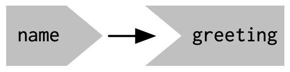{#fig-03-01 fig-alt="The graph consists of two blocks titled 'name' and 'greeting'. They are connected horizontally by an arrow from left tot the right. The left 'name' block has a pike to the right which would fit into the bump of the 'greeting' block." fig-align="center" width="8cm"}The reactive graph contains one symbol for every input and output, and we connect an input to an output whenever the output accesses the input. This graph tells you that greeting will need to be recomputed whenever name is changed. We’ll often describe this relationship as `greeting` has a `r glossary("reactive dependencies", "reactive dependency")` on `name`.Note the graphical conventions we used for the inputs and outputs: the name input naturally fits into the greeting output.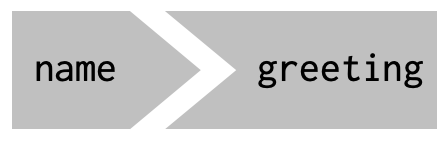{#fig-03-02 fig-alt="The graph consists of two blocks titled 'name' and 'greeting'. The left 'name' block has a pike to the right which fits into the bump of the 'greeting' block." fig-align="center" width="35%"}The reactive graph is a powerful tool for understanding how your app works. As your app gets more complicated, it’s often useful to make a quick high-level sketch of the reactive graph to remind you how all the pieces fit together. Throughout this book we’ll show you the reactive graph to help understand how the examples work, and later on, in @sec-chap14, you’ll learn how to use {**reactlog**} which will draw the graph for you.### Reactive expressions {#sec-03-reactive-expressions-sub}There’s one more important component that you’ll see in the reactive graph: the reactive expression. We’ll come back to reactive expressions in detail very shortly; for now think of them as a tool that reduces duplication in your reactive code by introducing additional nodes into the reactive graph.We don’t need a reactive expression in our very simple app, but I’ll add one anyway so you can see how it affects the reactive graph (see @fig-03-03).:::::{.my-r-code}:::{.my-r-code-header}:::::: {#cnj-03-greeting-example}: Interactive greeting as an example for reactive programming:::::::::::::{.my-r-code-container}::: {#lst-03-greeting-example2}```{r}#| label: greeting-example2#| eval: falseui <- shiny::fluidPage( shiny::textInput("name", "What's your name?"), shiny::textOutput("greeting"))server <-function(input, output, session) { output$greeting <- shiny::renderText(string()) string <- shiny::reactive(paste0("Hello ", input$name, "!"))}shiny::shinyApp(ui, server)```:::```{shinylive-r}#| standalone: trueui<- shiny::fluidPage(shiny::textInput("name","What's your name?"),shiny::textOutput("greeting"))server<- function(input, output, session){string<- shiny::reactive(paste0("Hello ", input$name, "!"))output$greeting<- shiny::renderText(string())}shiny::shinyApp(ui, server)```***Compare the tiny difference in the server code with @lst-03-greeting-example.:::::::::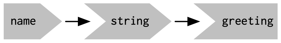{#fig-03-03 fig-alt="The graph consists of three blocks titled 'name', 'string and 'greeting'. The blocks are connected by two arrows from left to the right. 'name' block has a pike to the right which fits into the bump of the 'string' block which itself has a bump fitting into the 'greeting' block." fig-align="center" width="70%"}Reactive expressions take inputs and produce outputs so they have a shape that combines features of both inputs and outputs.### Execution orderIt’s important to understand that the order in which your code runs is solely determined by the reactive graph. This is different from most R code where the execution order is determined by the order of lines. For example, we could flip the order of the two lines in our simple server function::::::{.my-r-code}:::{.my-r-code-header}:::::: {#cnj-03-greeting-example}: Interactive greeting as an example for reactive programming:::::::::::::{.my-r-code-container}::: {#lst-03-greeting-example3}```{r}#| label: greeting-example3#| eval: falseui <- shiny::fluidPage( shiny::textInput("name", "What's your name?"), shiny::textOutput("greeting"))server <-function(input, output, session) { string <- shiny::reactive(paste0("Hello ", input$name, "!")) output$greeting <- shiny::renderText(string())}shiny::shinyApp(ui, server)```:::```{shinylive-r}#| standalone: trueui<- shiny::fluidPage(shiny::textInput("name","What's your name?"),shiny::textOutput("greeting"))server<- function(input, output, session){output$greeting<- shiny::renderText(string())string<- shiny::reactive(paste0("Hello ", input$name, "!"))}shiny::shinyApp(ui, server)```***Again: Compare the tiny difference in the server code; this time with @lst-03-greeting-example2.:::::::::You might think that this would yield an error because `output$greeting` refers to a reactive expression, string, that hasn’t been created yet. But remember Shiny is lazy, so that code is only run when the session starts, after string has been created.Instead, this code yields the same reactive graph as above, so the order in which the code is run is exactly the same. Organizing your code like this is confusing for humans, and best avoided. Instead, make sure that reactive expressions and outputs only refer to things defined above, not below. This will make your code easier to understand.This concept is very important and different to most other R code, so I’ll say it again:::: {.callout-important}The order in which reactive code is run is determined only by the reactive graph, not by its layout in the server function.:::### Exercises#### Find bugs:::::{.my-exercise}:::{.my-exercise-header}:::::: {#exr-03-ex-01-find-bugs}: Find the bugs in the three server functions:::::::::::::{.my-exercise-container}::: {.panel-tabset}###### Challenge:::::{.my-r-code}:::{.my-r-code-header}:::::: {#cnj-03-ex-01-find-bugs-challenge}: Find the bugs in the three server functions:::::::::::::{.my-r-code-container}Fix the simple errors found in each of the three server functions below. First try spotting the problem just by reading the code; then run the code to make sure you’ve fixed it.```{r}#| label: find-bugs-challenge#| eval: false#| code-fold: showlibrary(shiny)ui <-fluidPage(textInput("name", "What's your name?"),textOutput("greeting"))server1 <-function(input, output, server) { input$greeting <-renderText(paste0("Hello ", name))}server2 <-function(input, output, server) { greeting <-paste0("Hello ", input$name) output$greeting <-renderText(greeting)}server3 <-function(input, output, server) { output$greting <-paste0("Hello", input$name)}shinyApp(ui, server)```:::::::::###### Solution (Code):::::{.my-r-code}:::{.my-r-code-header}:::::: {#cnj-03-ex-01-find-bugs-solution-code}: Show the bugs in the three server functions and add correct code:::::::::::::{.my-r-code-container}::: {#lst-03-ex-01-find-bugs-solution-code}```{r}#| label: find-bugs-solution#| eval: false#| code-fold: showlibrary(shiny)ui <-fluidPage(textInput("name", "What's your name?"),textOutput("greeting"))# server1 <- function(input, output, server) {# input$greeting <- renderText(paste0("Hello ", name))##### output$greeting instead of input$greeting ######## }# # server2 <- function(input, output, server) {# greeting <- paste0("Hello ", input$name)##### assigning value directly not allowed ####### output$greeting <- renderText(greeting)# }# # server3 <- function(input, output, server) {# output$greting <- paste0("Hello", input$name)##### missing 'e' in output$greting ######## }# correct codeserver <-function(input, output, server) { output$greeting <-renderText(paste0("Hello", input$name))}shinyApp(ui, server)```::::::::::::###### Solution (Shiny):::::{.my-solution}:::{.my-solution-header}:::::: {#sol-03-ex-01-find-bugs-app-shiny}: Run @lst-03-ex-01-find-bugs-solution-code with correct code:::::::::::::{.my-solution-container}```{shinylive-r}#| standalone: true#| viewerHeight: 100library(shiny)ui<- fluidPage(textInput("name","What's your name?"),textOutput("greeting"))# server1 <- function(input, output, server) {# input$greeting <- renderText(paste0("Hello ", name))##### output$greeting instead of input$greeting ######## }# # server2 <- function(input, output, server) {# greeting <- paste0("Hello ", input$name)##### assigning value directly not allowed ####### output$greeting <- renderText(greeting)# }# # server3 <- function(input, output, server) {# output$greting <- paste0("Hello", input$name)##### missing 'e' in output$greting ######## }# correct codeserver<- function(input, output, server){output$greeting<- renderText(paste0("Hello", input$name))}shinyApp(ui, server)```:::::::::::::::::::::#### Draw reactive graphs:::::{.my-exercise}:::{.my-exercise-header}:::::: {#exr-03-ex-02-draw-reactive-graphs}: Draw reactive graph for server functions:::::::::::::{.my-exercise-container}::: {.panel-tabset}###### Challenge:::::{.my-r-code}:::{.my-r-code-header}:::::: {#cnj-03-ex-02-find-bugs-challenge}: Draw reactive graph for server functions:::::::::::::{.my-r-code-container}::: {#lst-03-draw-graphs-challenge}```{r}#| label: draw-graphs-challenge#| eval: false#| code-fold: showserver1 <-function(input, output, session) { c <-reactive(input$a + input$b) e <-reactive(c() + input$d) output$f <-renderText(e())}server2 <-function(input, output, session) { x <-reactive(input$x1 + input$x2 + input$x3) y <-reactive(input$y1 + input$y2) output$z <-renderText(x() /y())}server3 <-function(input, output, session) { d <-reactive(c() ^ input$d) a <-reactive(input$a *10) c <-reactive(b() / input$c) b <-reactive(a() + input$b)}```::::::::::::###### Solution (Graphs):::::{.my-r-code}:::{.my-r-code-header}:::::: {#cnj-03-ex-02-draw-graphs-solution}: Draw the graphs in the three server functions of @lst-03-draw-graphs-challenge:::::::::::::{.my-r-code-container}I've tried to find the solution myself and then I've compared my result with the [drawing graph solutions](https://mastering-shiny-solutions.org/basic-reactivity.html#solution-15) in Mastering Shiny Solutions [@ther4dsonlinelearningcommunity2023]The first two examples of my trials coincide with Mastering Shiny Solutions. In the third example I had a chain of the inputs a,b,c,d and not — as in Mastering Shiny Solutions — a step by step chain where each input is depending of an input with the same name.***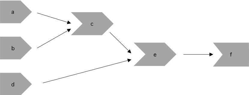{#fig-03-04fig-alt="The graph consists of six blocks titled a-f. 'a' and 'b' are connected horizontally by an arrow from left tot the right with 'c'. The block 'e' gets its input (= arrows) by 'c' and 'd' and 'e' finally put its result into 'f'" fig-align="center" width="50%"}***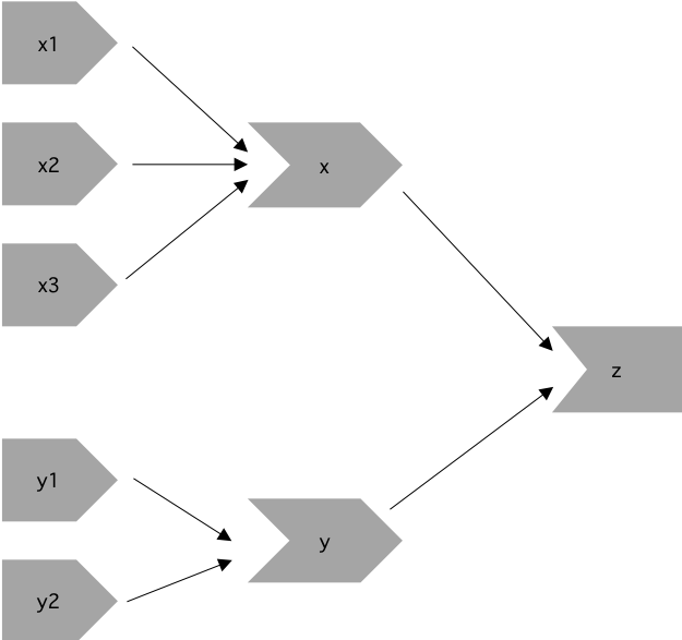{#fig-03-05 fig-alt="The graph consists of six blocks titled a-f. 'a' and 'b' are connected horizontally by an arrow from left tot the right with 'c'. The block 'e' gets its input (= arrows) by 'c' and 'd' and 'e' finally put its result into 'f'" fig-align="center" width="50%"}***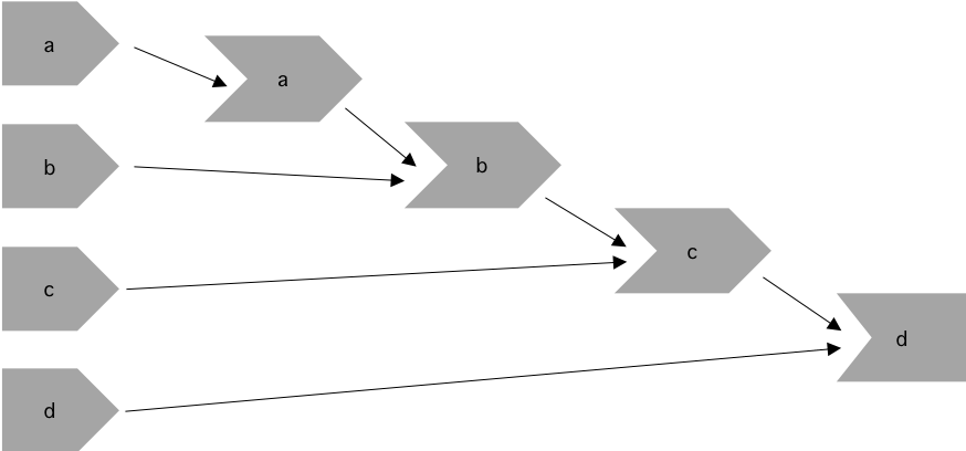{#fig-03-06 fig-alt="The graph consists of six blocks titled a-f. 'a' and 'b' are connected horizontally by an arrow from left tot the right with 'c'. The block 'e' gets its input (= arrows) by 'c' and 'd' and 'e' finally put its result into 'f'" fig-align="center" width="50%"}:::::::::Compare the graphs with the server code snippets in @lst-03-draw-graphs-challenge.::::::::::::#### Failed code snippet:::::{.my-exercise}:::{.my-exercise-header}:::::: {#exr-03-ex-03-failed-code}: Why will this code fail?:::::::::::::{.my-exercise-container}::: {.panel-tabset}###### Challenge:::::{.my-r-code}:::{.my-r-code-header}:::::: {#cnj-03-ex-03-failed-code-challenge}: Why will this code snippet fail?:::::::::::::{.my-r-code-container}::: {#lst-03-ex-03-failed-code-challenge}```{r}#| label: failed-code-challenge#| eval: false#| code-fold: showvar <-reactive(df[[input$var]])range <-reactive(range(var(), na.rm =TRUE))```Failed code snippet::::::::::::###### Solution (Code):::::{.my-r-code}:::{.my-r-code-header}:::::: {#cnj-03-ex-03-failed-code-solution}: Why failed the code in @lst-03-ex-03-failed-code-challenge:::::::::::::{.my-r-code-container}::: {#lst-03-ex-03-failed-code-solution}```{r}#| label: failed-code-solution#| eval: false#| code-fold: showlibrary(shiny)df <- mtcarsui <-fluidPage(selectInput("var", NULL, choices =colnames(df)),verbatimTextOutput("debug"))server <-function(input, output, session) { col_var <-reactive( df[input$var] ) col_range <-reactive({ range(col_var(), na.rm =TRUE ) }) output$debug <-renderPrint({ col_range() })}shinyApp(ui = ui, server = server)```Code example with changed names of the reactives::::::::::::###### Solution (Shiny):::::{.my-solution}:::{.my-solution-header}:::::: {#sol-03-ex-01-find-bugs-app-shiny}: Run @lst-03-ex-03-failed-code-challenge with correct code:::::::::::::{.my-solution-container}base::range() and stats::var() are bad names for reactives because they are reserved names for other functions:- `base::range()` returns a vector containing the minimum and maximum of all the given arguments.- `stats::var()` computes the variance of x.In the following solution code from [Mastering Shiny Solutions](https://mastering-shiny-solutions.org/basic-reactivity.html#solution-16) I have followed their idea to change `range` into `col_range` and `var` into `col_var`. These new names substitute the bad names for the reactives in the failed code snippet.```{shinylive-r}#| standalone: true#| viewerHeight: 300library(shiny)df<- mtcarsui<- fluidPage(selectInput("var", NULL, choices = colnames(df)),verbatimTextOutput("debug"))server<- function(input, output, session){col_var<- reactive(df[input$var])col_range<- reactive({range(col_var(), na.rm = TRUE )})output$debug<- renderPrint({col_range()})}shinyApp(ui = ui, server = server)```:::::::::Compare the Shiny result with the code used for the solution in @lst-03-ex-03-failed-code-solution.::::::::::::## Reactive expressions {#sec-03-reactive-expressions}Reactive expressions have a flavor of both inputs and outputs:- Like outputs, reactive expressions depend on inputs and automatically know when they need updating.- Like inputs, you can use the results of a reactive expression in an output.This duality means we need some new vocab: I’ll use **producers** to refer to reactive inputs and expressions, and **consumers** to refer to reactive expressions and outputs.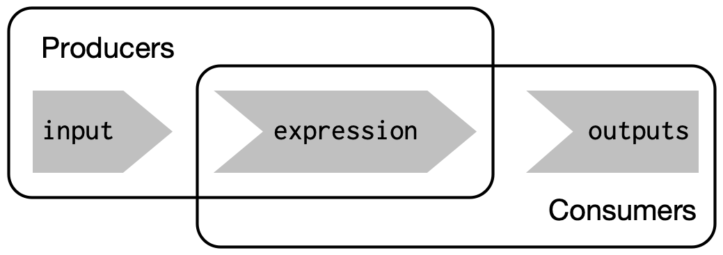{#fig-03-07fig-alt="The graphics shows the connection between `input`, `expression` and `outputs` as Venn diagram. `input` and `expression` form the so-called **Producers**; `expression` and `outputs` constitute the **Consumers**" fig-align="center" width="70%"}### The motivationImagine I want to compare two simulated datasets with a plot and a hypothesis test. I’ve done a little experimentation and come up with the functions below: `freqpoly()` visualizes the two distributions with `r glossary("frequency polygon")`s, and `t_test()` uses a t-test to compare means and summarizes the results with a string::::::{.my-r-code}:::{.my-r-code-header}:::::: {#cnj-03-compare-simulated-datasets}: Compare two simulated datasets with a plot and a hypothesis test.:::::::::::::{.my-r-code-container}```{r}#| label: fig-compare-simulated-datasets#| fig-cap: "Compare two simulated datasets with a plot and a hypothesis test"freqpoly <-function(x1, x2, binwidth =0.1, xlim =c(-3, 3)) { df <- base::data.frame(x = base::c(x1, x2),g = base::c(base::rep("x1", base::length(x1)), base::rep("x2", base::length(x2))) ) ggplot2::ggplot(df, ggplot2::aes(x, colour = g)) + ggplot2::geom_freqpoly(binwidth = binwidth, linewidth =1) + ggplot2::coord_cartesian(xlim = xlim)}t_test <-function(x1, x2) { test <- stats::t.test(x1, x2)# use sprintf() to format t.test() results compactly base::sprintf("p value: %0.3f\n[%0.2f, %0.2f]", test$p.value, test$conf.int[1], test$conf.int[2] )}### prepare valuesx1 <- stats::rnorm(100, mean =0, sd =0.5)x2 <- stats::rnorm(200, mean =0.15, sd =0.9)### call functionsfreqpoly(x1, x2)base::cat(t_test(x1, x2))```:::::::::### The appI’d like to use these two tools to quickly explore a bunch of simulations. A Shiny app is a great way to do this because it lets you avoid tediously modifying and re-running R code. Below I wrap the pieces into a Shiny app where I can interactively tweak the inputs.::: {.my-code-collection}:::: {.my-code-collection-header}::::: {.my-code-collection-icon}::::::::::: {#exm-03-compare-simulated-data}: Case study: Compare simulated data V1::::::::::::::{.my-code-collection-container}::: {.panel-tabset}###### Code:::::{.my-r-code}:::{.my-r-code-header}:::::: {#cnj-03-compare-simulated-data-code}: Case study: Compare simulated data V1:::::::::::::{.my-r-code-container}::: {#lst-03-compare-simulated-data-code1}```{r}#| label: compare-simulated-data-code#| eval: false## source .R file with the two functions didn't work## so I had to use the original code instead of the followingbase::source( base::paste0(here::here(), "/R/shiny-03-V2.R"),local =TRUE,chdir =TRUE,encoding ="utf-8" )library(shiny)library(ggplot2)library(munsell)ui <-fluidPage(fluidRow(column(4,"Distribution 1",numericInput("n1", label ="n", value =1000, min =1),numericInput("mean1", label ="µ", value =0, step =0.1),numericInput("sd1", label ="σ", value =0.5, min =0.1, step =0.1) ),column(4,"Distribution 2",numericInput("n2", label ="n", value =1000, min =1),numericInput("mean2", label ="µ", value =0, step =0.1),numericInput("sd2", label ="σ", value =0.5, min =0.1, step =0.1) ),column(4,"Frequency polygon",numericInput("binwidth", label ="Bin width", value =0.1, step =0.1),sliderInput("range", label ="range", value =c(-3, 3), min =-5, max =5) ) ),fluidRow(column(9, plotOutput("hist")),column(3, verbatimTextOutput("ttest")) ))server <-function(input, output, session) { output$hist <-renderPlot({ x1 <-rnorm(input$n1, input$mean1, input$sd1) x2 <-rnorm(input$n2, input$mean2, input$sd2)freqpoly(x1, x2, binwidth = input$binwidth, xlim = input$range) }, res =96) output$ttest <-renderText({ x1 <-rnorm(input$n1, input$mean1, input$sd1) x2 <-rnorm(input$n2, input$mean2, input$sd2)t_test(x1, x2) })}shinyApp(ui, server)```Compare simulated data with plot and t-test::::::::::::###### Shiny:::::{.my-r-code}:::{.my-r-code-header}:::::: {#cnj-03-compare-simulated-data-shiny}: Case study: Compare simulated data V1:::::::::::::{.my-r-code-container}```{shinylive-r}#| standalone: true#| viewerHeight: 600library(shiny)library(ggplot2)library(munsell)# source .R file with the two functions didn't workfreqpoly<- function(x1, x2, binwidth = 0.1, xlim = c(-3, 3)){df<- base::data.frame(x = base::c(x1, x2),g = base::c(base::rep("x1", base::length(x1)),base::rep("x2", base::length(x2))))ggplot2::ggplot(df, ggplot2::aes(x, colour = g))+ggplot2::geom_freqpoly(binwidth = binwidth, linewidth = 1)+ggplot2::coord_cartesian(xlim = xlim)}t_test<- function(x1, x2){test<- stats::t.test(x1, x2)# use sprintf() to format t.test() results compactlybase::sprintf("p value: %0.3f\n[%0.2f, %0.2f]",test$p.value, test$conf.int[1], test$conf.int[2])}# base::source(# base::paste0(here::here(), "/R/shiny-03-V2.R"),# local = TRUE,# chdir = TRUE,# encoding = "utf-8"# )ui<- fluidPage(fluidRow(column(4,"Distribution 1",numericInput("n1", label = "n", value = 1000, min = 1),numericInput("mean1", label = "µ", value = 0, step = 0.1),numericInput("sd1", label = "σ", value = 0.5, min = 0.1, step = 0.1)),column(4,"Distribution 2",numericInput("n2", label = "n", value = 1000, min = 1),numericInput("mean2", label = "µ", value = 0, step = 0.1),numericInput("sd2", label = "σ", value = 0.5, min = 0.1, step = 0.1)),column(4,"Frequency polygon",numericInput("binwidth", label = "Bin width", value = 0.1, step = 0.1),sliderInput("range", label = "range", value = c(-3, 3), min = -5, max = 5))),fluidRow(column(9, plotOutput("hist")),column(3, verbatimTextOutput("ttest"))))server<- function(input, output, session){output$hist<- renderPlot({x1<- rnorm(input$n1, input$mean1, input$sd1)x2<- rnorm(input$n2, input$mean2, input$sd2)freqpoly(x1, x2, binwidth = input$binwidth, xlim = input$range)}, res = 96)output$ttest<- renderText({x1<- rnorm(input$n1, input$mean1, input$sd1)x2<- rnorm(input$n2, input$mean2, input$sd2)t_test(x1, x2)})}shinyApp(ui, server)```:::::::::Compare the code in @lst-03-compare-simulated-data-code1 for this shiny app.::::::::::::::: {.callout-warning}I had to duplicate the code for the two functions `freqpoly()`and`t_test()`because sourcing the code from an extra .R file did not work. I tried several options of `source("path-to-file", local = TRUE)`- file in an extra directory with additional option `chdir = TRUE`,- file in main directory references with `source('./<file_name>', local=TRUE)`- file calling with `here::here()`applying`if(FALSE){library(here)}`to include additional R packages that are not automatically discovered,- adding `encoding="utf-8"`:::You can find a live version at <https://hadley.shinyapps.io/ms-case-study-1>;I recommend opening the app with the above link, because it uses the whole screen width and it is therefore easier to play with. Having a quick play to make sure you understand its basic operation is essential before you continue reading.### The reactive graphShiny is smart enough to update an output only when the inputs it refers to change;it’s not smart enough to only selectively run pieces of code inside an output. In other words, outputs are atomic: they’re either executed or not as a whole.For example, take this snippet from the server:```x1<- rnorm(input$n1, input$mean1, input$sd1)x2<- rnorm(input$n2, input$mean2, input$sd2)t_test(x1, x2)```As a human reading this code you can tell that we only need to update `x1`when`n1`,`mean1`, or `sd1`changes, and we only need to update `x2`when`n2`,`mean2`, or `sd2`changes. Shiny, however, only looks at the output as a whole, so it will update both `x1`and`x2`every time one of `n1`,`mean1`,`sd1`,`n2`,`mean2`, or `sd2`changes. This leads to the reactive graph shown in @fig-03-08.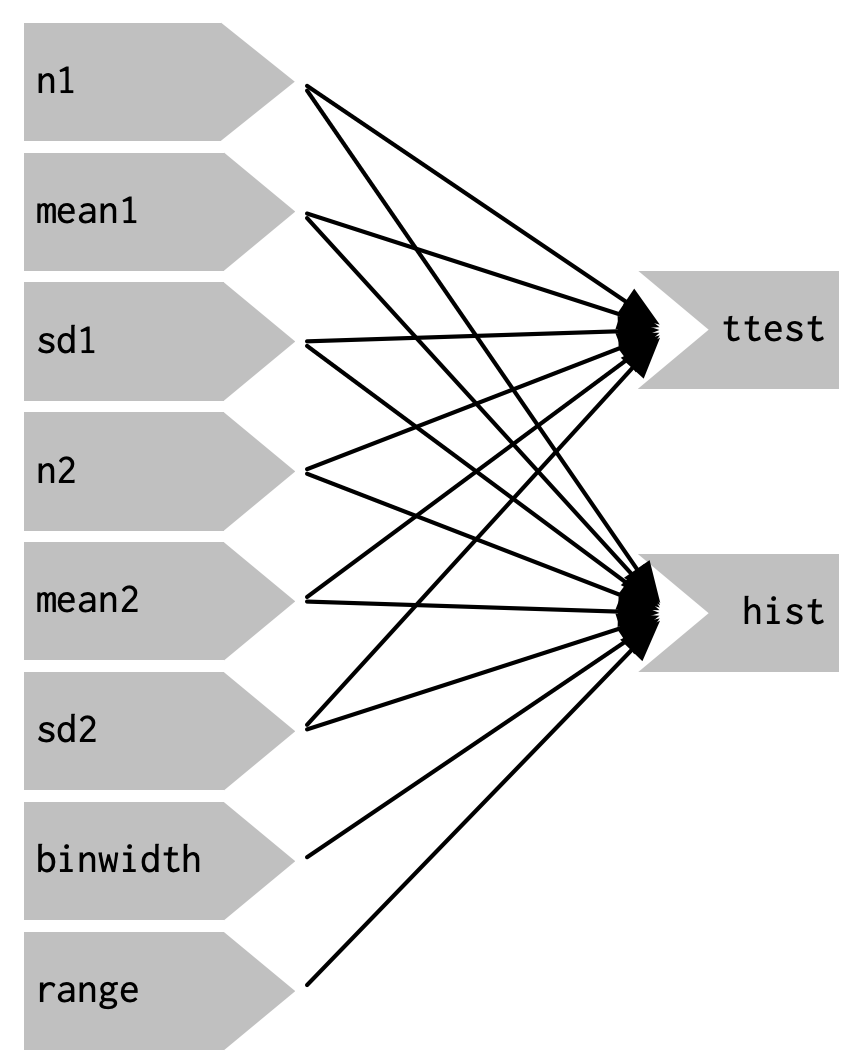{#fig-03-08fig-alt="The inputs n1, mean1, sd1, n2, mean2, sd2 are all connected to the outputs ttest and hist. Additionally binwidth and range are connected to hist." fig-align="center"width="40%"}You’ll notice that the graph is very dense: almost every input is connected directly to every output. This creates two problems:- The app is hard to understand because there are so many connections. There are no pieces of the app that you can pull out and analyse in isolation.- The app is inefficient because it does more work than necessary. For example, if you change the breaks of the plot, the data is recalculated;ifyou change the value of `n1`,`x2`is updated (intwo places!).There’s one other major flaw in the app: the frequency polygon and t-test use separate random draws. This is rather misleading, as you’d expect them to be working on the same underlying data.Fortunately, we can fix all these problems by using reactive expressions to pull out repeated computation.### Simplifying the graph::: {.my-code-collection}:::: {.my-code-collection-header}::::: {.my-code-collection-icon}::::::::::: {#exm-03-compare-simulated-data2}: Case study: Compare simulated data V2::::::::::::::{.my-code-collection-container}::: {.panel-tabset}###### Code:::::{.my-r-code}:::{.my-r-code-header}:::::: {#cnj-03-compare-simulated-data-code2}: Case study: Compare simulated data V2:::::::::::::{.my-r-code-container}::: {#lst-03-compare-simulated-data-code2}```{r}#| label: compare-simulated-data-code2#| eval: false## source .R file with the two functions didn't workbase::source(base::paste0(here::here(),"/R/shiny-03-V2.R"),local=TRUE,chdir = TRUE,encoding = "utf-8")library(shiny)library(ggplot2)library(munsell)ui<- fluidPage(fluidRow(column(4,"Distribution 1",numericInput("n1", label = "n", value = 1000, min = 1),numericInput("mean1", label = "µ", value = 0, step = 0.1),numericInput("sd1", label = "σ", value = 0.5, min = 0.1, step = 0.1)),column(4,"Distribution 2",numericInput("n2", label = "n", value = 1000, min = 1),numericInput("mean2", label = "µ", value = 0, step = 0.1),numericInput("sd2", label = "σ", value = 0.5, min = 0.1, step = 0.1)),column(4,"Frequency polygon",numericInput("binwidth", label = "Bin width", value = 0.1, step = 0.1),sliderInput("range", label = "range", value = c(-3, 3), min = -5, max = 5))),fluidRow(column(9, plotOutput("hist")),column(3, verbatimTextOutput("ttest"))))server<- function(input, output, session){x1<- reactive(rnorm(input$n1, input$mean1, input$sd1))x2<- reactive(rnorm(input$n2, input$mean2, input$sd2))output$hist<- renderPlot({freqpoly(x1(), x2(), binwidth = input$binwidth, xlim = input$range)}, res = 96)output$ttest<- renderText({t_test(x1(), x2())})}shinyApp(ui, server)```Compare simulated data with plot and t-test using reactive expressions:::Compare the code in @lst-03-compare-simulated-data-code1 for this shiny app without reactive expressions:::::::::###### Shiny:::::{.my-r-code}:::{.my-r-code-header}:::::: {#cnj-03-compare-simulated-data-shiny2}: Case study: Compare simulated data V2:::::::::::::{.my-r-code-container}```{shinylive-r}#| standalone: true#| viewerHeight: 600# source .R file with the two functions didn't workfreqpoly<- function(x1, x2, binwidth = 0.1, xlim = c(-3, 3)){df<- base::data.frame(x = base::c(x1, x2),g = base::c(base::rep("x1", base::length(x1)),base::rep("x2", base::length(x2))))ggplot2::ggplot(df, ggplot2::aes(x, colour = g))+ggplot2::geom_freqpoly(binwidth = binwidth, linewidth = 1)+ggplot2::coord_cartesian(xlim = xlim)}t_test<- function(x1, x2){test<- stats::t.test(x1, x2)# use sprintf() to format t.test() results compactlybase::sprintf("p value: %0.3f\n[%0.2f, %0.2f]",test$p.value, test$conf.int[1], test$conf.int[2])}# base::source(# base::paste0(here::here(), "/R/shiny-03-V2.R"),# local = TRUE,# chdir = TRUE,# encoding = "utf-8"# )library(shiny)library(ggplot2)library(munsell)ui<- fluidPage(fluidRow(column(4,"Distribution 1",numericInput("n1", label = "n", value = 1000, min = 1),numericInput("mean1", label = "µ", value = 0, step = 0.1),numericInput("sd1", label = "σ", value = 0.5, min = 0.1, step = 0.1)),column(4,"Distribution 2",numericInput("n2", label = "n", value = 1000, min = 1),numericInput("mean2", label = "µ", value = 0, step = 0.1),numericInput("sd2", label = "σ", value = 0.5, min = 0.1, step = 0.1)),column(4,"Frequency polygon",numericInput("binwidth", label = "Bin width", value = 0.1, step = 0.1),sliderInput("range", label = "range", value = c(-3, 3), min = -5, max = 5))),fluidRow(column(9, plotOutput("hist")),column(3, verbatimTextOutput("ttest"))))server<- function(input, output, session){x1<- reactive(rnorm(input$n1, input$mean1, input$sd1))x2<- reactive(rnorm(input$n2, input$mean2, input$sd2))output$hist<- renderPlot({freqpoly(x1(), x2(), binwidth = input$binwidth, xlim = input$range)}, res = 96)output$ttest<- renderText({t_test(x1(), x2())})}shinyApp(ui, server)```:::::::::Compare the code in @lst-03-compare-simulated-data-code2 for this shiny app.::::::::::::This transformation yields the substantially simpler graph shown in @fig-03-09. This simpler graph makes it easier to understand the app because you can understand connected components in isolation;the values of the distribution parameters only affect the output via `x1`and`x2.`This rewrite also makes the app much more efficient since it does much less computation. Now, when you change the `binwidth`or`range`, only the plot changes, not the underlying data.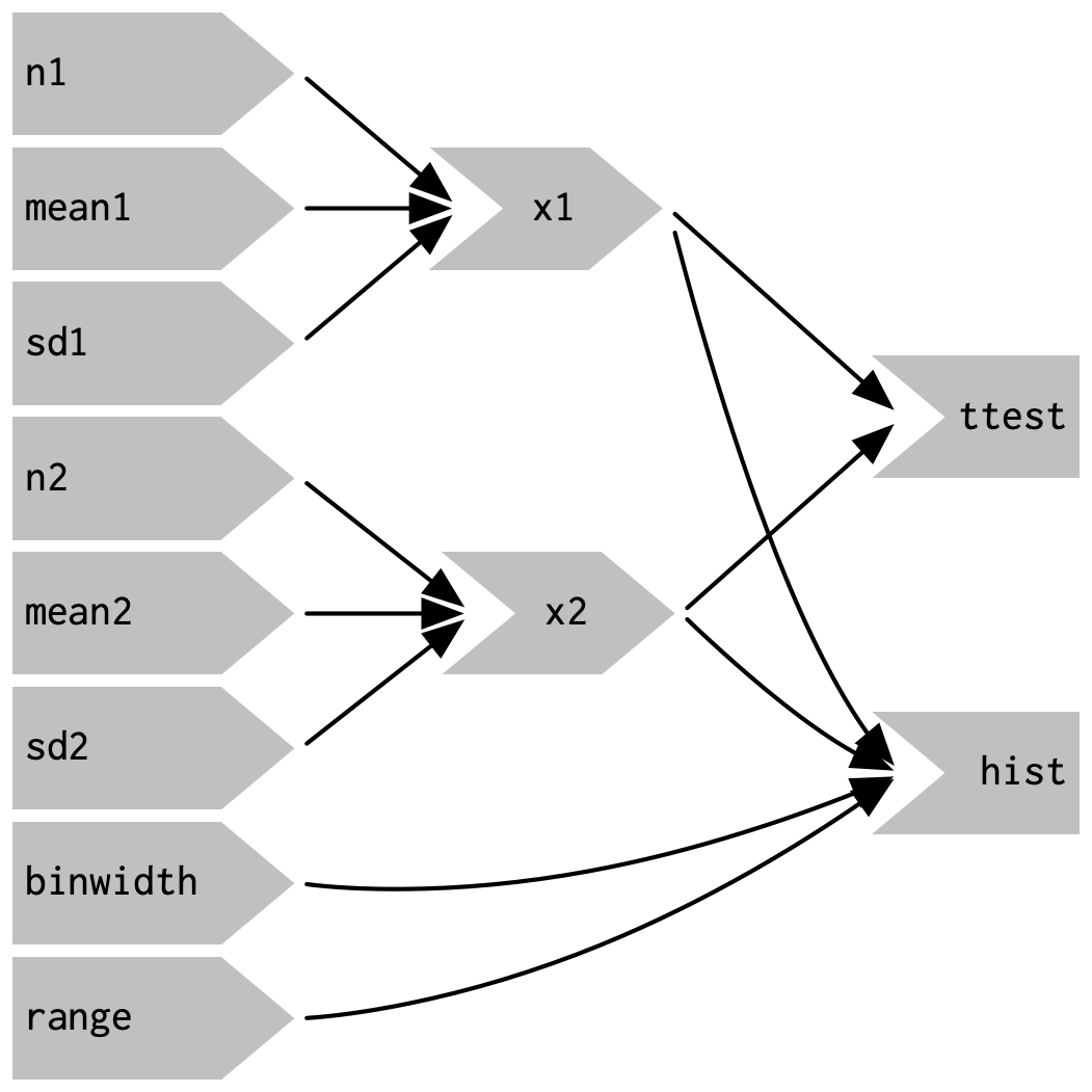{#fig-03-09fig-alt="The inputs n1, mean1, sd1 connect to x1 and the inputs n2, mean2, sd2 connect to x2. x1 and x2 connect to ttest and hist. binwidth and range connect to hist." fig-align="center"width="40%"}To emphasize this modularity @fig-03-10 draws boxes around the independent components. We’ll come back to this idea in @sec-chap19, when we discuss modules. Modules allow you to extract out repeated code for reuse, while guaranteeing that it’s isolated from everything else in the app. Modules are an extremely useful and powerful technique for more complex apps.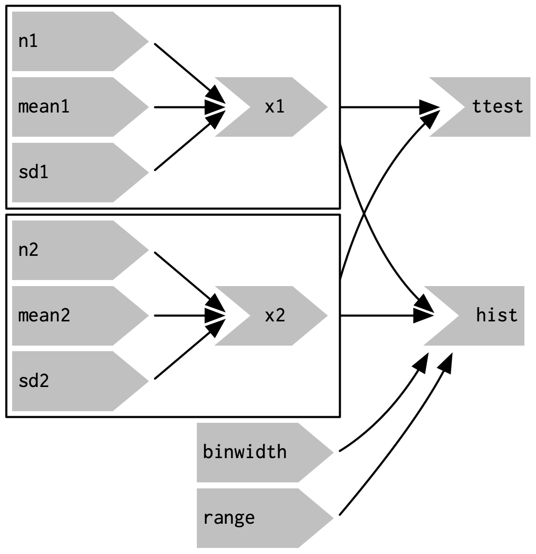{#fig-03-10fig-alt="The inputs n1, mean1, sd1 connect to x1; the inputs n2, mean2, sd2 connect to x2. x1 and x2 connect to ttest and hist; binwidth and range connect to hist. Additionally there are two boxes drawn. One around n1, mean, sd1 and x1, the other one around n2, mean2, sd2 and x2." fig-align="center"width="40%"}You might be familiar with the “rule of three” of programming: whenever you copy and paste something three times, you should figure out how to reduce the duplication (typically by writing a function). [In Shiny, however, you should consider the rule of one]{.mark}: whenever you copy and paste something once, you should consider extracting the repeated code out into a reactive expression. The rule is stricter for Shiny because reactive expressions don’t just make it easier for humans to understand the code, they also improve Shiny’s ability to efficiently rerun code.### Why do we need reactive expressions?When you first start working with reactive code, you might wonder why we need reactive expressions. Why can’t you use your existing tools for reducing duplication in code: creating new variables and writing functions? Unfortunately neither of these techniques work in a reactive environment.-**If you try to use a variable to reduce duplication**, you’ll get an error because you’re attempting to access input values outside of a reactive context. Even if you didn’t get that error, you’d still have a problem: `x1`and`x2`would only be computed once, when the session begins, not every time one of the inputs was updated.-**If you try to use a function to reduce duplication** it has the same problem as the original code: any input will cause all outputs to be recomputed, and the t-test and the frequency polygon will be run on separate samples. Reactive expressions automatically cache their results, and only update when their inputs change.## Controlling timing of evaluation {#sec-03-control-timing}Now that you’re familiar with the basic ideas of reactivity, we’ll discuss two more advanced techniques that allow you to either increase or decrease how often a reactive expression is executed. Here I’ll show how to use the basic techniques;in@sec-chap15, we’ll come back to their underlying implementations.To explore the basic ideas, I’m going to simplify my simulation app. I’ll use a distribution with only one parameter, and force both samples to share the same `n`. I’ll also remove the plot controls. This yields a smaller UI object and server function.::: {.my-code-collection}:::: {.my-code-collection-header}::::: {.my-code-collection-icon}::::::::::: {#exm-03-compare-simulated-data3}: Case study: Compare simulated data V3::::::::::::::{.my-code-collection-container}::: {.panel-tabset}###### Code:::::{.my-r-code}:::{.my-r-code-header}:::::: {#cnj-03-compare-simulated-data-code3}: Case study: Compare simulated data V3:::::::::::::{.my-r-code-container}::: {#lst-03-compare-simulated-data-code3}```{r}#| label: compare-simulated-data-code3#| eval: false## source .R file with the two functions didn't workbase::source(base::paste0(here::here(),"/R/shiny-03-V2.R"),local=TRUE,chdir = TRUE,encoding = "utf-8")library(shiny)library(ggplot2)library(munsell)ui<- fluidPage(fluidRow(column(3,numericInput("lambda1", label = "lambda1", value = 3),numericInput("lambda2", label = "lambda2", value = 5),numericInput("n", label = "n", value = 1e4, min = 0)),column(9, plotOutput("hist"))))server<- function(input, output, session){x1<- reactive(rpois(input$n, input$lambda1))x2<- reactive(rpois(input$n, input$lambda2))output$hist<- renderPlot({freqpoly(x1(), x2(), binwidth = 1, xlim = c(0, 40))}, res = 96)}shinyApp(ui, server)```A simpler app that displays a frequency polygon of random numbers drawn from two Poisson distributions.:::Compare the code with original app @lst-03-compare-simulated-data-code1 (without reactive expression)and @lst-03-compare-simulated-data-code2 (with reactive expressions)with this more simpler app that draws from two Poisson distributions.:::::::::###### Shiny:::::{.my-r-code}:::{.my-r-code-header}:::::: {#cnj-03-compare-simulated-data-shiny3}: Case study: Compare simulated data V3:::::::::::::{.my-r-code-container}```{shinylive-r}#| standalone: true#| viewerHeight: 600# source .R file with the two functions didn't workfreqpoly<- function(x1, x2, binwidth = 0.1, xlim = c(-3, 3)){df<- base::data.frame(x = base::c(x1, x2),g = base::c(base::rep("x1", base::length(x1)),base::rep("x2", base::length(x2))))ggplot2::ggplot(df, ggplot2::aes(x, colour = g))+ggplot2::geom_freqpoly(binwidth = binwidth, linewidth = 1)+ggplot2::coord_cartesian(xlim = xlim)}t_test<- function(x1, x2){test<- stats::t.test(x1, x2)# use sprintf() to format t.test() results compactlybase::sprintf("p value: %0.3f\n[%0.2f, %0.2f]",test$p.value, test$conf.int[1], test$conf.int[2])}# base::source(# base::paste0(here::here(), "/R/shiny-03-V2.R"),# local = TRUE,# chdir = TRUE,# encoding = "utf-8"# )library(shiny)library(ggplot2)library(munsell)ui<- fluidPage(fluidRow(column(3,numericInput("lambda1", label = "lambda1", value = 3),numericInput("lambda2", label = "lambda2", value = 5),numericInput("n", label = "n", value = 1e4, min = 0)),column(9, plotOutput("hist"))))server<- function(input, output, session){x1<- reactive(rpois(input$n, input$lambda1))x2<- reactive(rpois(input$n, input$lambda2))output$hist<- renderPlot({freqpoly(x1(), x2(), binwidth = 1, xlim = c(0, 40))}, res = 96)}shinyApp(ui, server)```:::::::::Compare the code in @lst-03-compare-simulated-data-code3 for this shiny app.:::To play around with this app use the live version at <https://hadley.shinyapps.io/ms-simulation-2>.:::::::::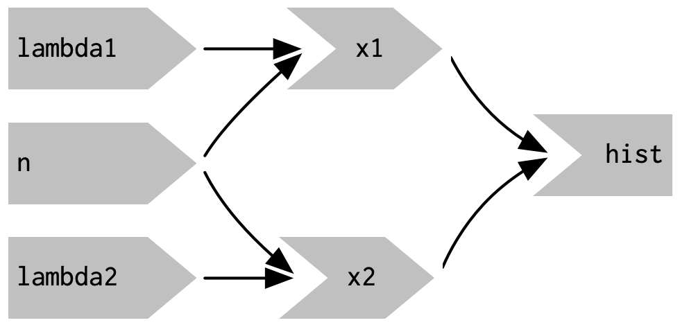{#fig-03-11fig-alt="lambda1 and n connect to x1, lambda2 and n connect to x2. x1 and x2 connect to the hist output." fig-align="center"width="40%"}### Timed invalidation {#sec-03-timed-invalidation}Imagine you wanted to reinforce the fact that this is for simulated data by constantly resimulating the data, so that you see an animation rather than a static plot. We can increase the frequency of updates with a new function: `shiny::reactiveTimer()`.`shiny::reactiveTimer()`is a reactive expression that has a dependency on a hidden input: the current time. You can use a `reactiveTimer()`when you want a reactive expression to invalidate itself more often than it otherwise would. For example, the following code uses an interval of 500 ms so that the plot will update twice a second. This is fast enough to remind you that you’re looking at a simulation, without dizzying you with rapid changes.::: {.my-code-collection}:::: {.my-code-collection-header}::::: {.my-code-collection-icon}::::::::::: {#exm-03-compare-simulated-data4}: Case study: Compare simulated data V4::::::::::::::{.my-code-collection-container}::: {.panel-tabset}###### Code:::::{.my-r-code}:::{.my-r-code-header}:::::: {#cnj-03-compare-simulated-data-code4}: Case study: Compare simulated data V4:::::::::::::{.my-r-code-container}::: {#lst-03-compare-simulated-data-code4}```{r}#| label: compare-simulated-data-code4#| eval: false# source .R file with the two functions didn't workbase::source(base::paste0(here::here(),"/R/shiny-03-V2.R"),local=TRUE,chdir = TRUE,encoding = "utf-8")library(shiny)library(ggplot2)library(munsell)ui<- fluidPage(fluidRow(column(3,numericInput("lambda1", label = "lambda1", value = 3),numericInput("lambda2", label = "lambda2", value = 5),numericInput("n", label = "n", value = 1e4, min = 0)),column(9, plotOutput("hist"))))server<- function(input, output, session){timer<- reactiveTimer(500)x1<- reactive({timer()rpois(input$n, input$lambda1)})x2<- reactive({timer()rpois(input$n, input$lambda2)})output$hist<- renderPlot({freqpoly(x1(), x2(), binwidth = 1, xlim = c(0, 40))}, res = 96)}shinyApp(ui, server)```Animation of a frequency polygon of random numbers drawn from two Poisson distributions.:::Note how we use `timer()`inthe reactive expressions that compute `x1()`and`x2()`: we call it, but don’t use the value. This lets `x1`and`x2`take a reactive dependency on timer, without worrying about exactly what value it returns.Compare the code with static app @lst-03-compare-simulated-data-code3 with this animation.:::::::::###### Shiny:::::{.my-r-code}:::{.my-r-code-header}:::::: {#cnj-03-compare-simulated-data-shiny4}: Case study: Compare simulated data V4:::::::::::::{.my-r-code-container}```{shinylive-r}#| standalone: true#| viewerHeight: 600# source .R file with the two functions didn't workfreqpoly<- function(x1, x2, binwidth = 0.1, xlim = c(-3, 3)){df<- base::data.frame(x = base::c(x1, x2),g = base::c(base::rep("x1", base::length(x1)),base::rep("x2", base::length(x2))))ggplot2::ggplot(df, ggplot2::aes(x, colour = g))+ggplot2::geom_freqpoly(binwidth = binwidth, linewidth = 1)+ggplot2::coord_cartesian(xlim = xlim)}t_test<- function(x1, x2){test<- stats::t.test(x1, x2)# use sprintf() to format t.test() results compactlybase::sprintf("p value: %0.3f\n[%0.2f, %0.2f]",test$p.value, test$conf.int[1], test$conf.int[2])}# source(# paste0(here::here(), "/R/shiny-03-V2.R"),# local = TRUE,# chdir = TRUE,# encoding = "utf-8"# )library(shiny)library(ggplot2)library(munsell)ui<- fluidPage(fluidRow(column(3,numericInput("lambda1", label = "lambda1", value = 3),numericInput("lambda2", label = "lambda2", value = 5),numericInput("n", label = "n", value = 1e4, min = 0)),column(9, plotOutput("hist"))))server<- function(input, output, session){timer<- reactiveTimer(500)x1<- reactive({timer()rpois(input$n, input$lambda1)})x2<- reactive({timer()rpois(input$n, input$lambda2)})output$hist<- renderPlot({freqpoly(x1(), x2(), binwidth = 1, xlim = c(0, 40))}, res = 96)}shinyApp(ui, server)```:::::::::Compare the code in @lst-03-compare-simulated-data-code3 for this shiny app.::::::::::::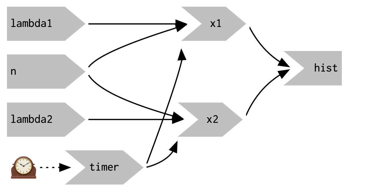{#fig-03-12fig-alt="lambda1 and n connect to x1, lambda2 and n connect to x2. x1 and x2 connect to the hist output. Additionally there is a (hidden) timer input that connects to x1 and x2." fig-align="center"width="50%"}### On clickIn the above scenario, think about what would happen if the simulation code took 1 second to run. We perform the simulation every 0.5s, so Shiny would have more and more to do, and would never be able to catch up. The same problem can happen if someone is rapidly clicking buttons in your app and the computation you are doing is relatively expensive. It’s possible to create a big backlog of work for Shiny, and while it’s working on the backlog, it can’t respond to any new events. This leads to a poor user experience.If this situation arises in your app, you might want to require the user to opt-in to performing the expensive calculation by requiring them to click a button. This is a great use case for an `shiny::actionButton()`.::: {.my-code-collection}:::: {.my-code-collection-header}::::: {.my-code-collection-icon}::::::::::: {#exm-03-compare-simulated-data5-action-button}: Case study: Compare simulated data V5 (action button V1)::::::::::::::{.my-code-collection-container}::: {.panel-tabset}###### Code:::::{.my-r-code}:::{.my-r-code-header}:::::: {#cnj-03-compare-simulated-data-code5-action-button1}: Case study: Compare simulated data V5 (action button V1):::::::::::::{.my-r-code-container}::: {#lst-03-compare-simulated-data-code5-action-button1}```{r}#| label: compare-simulated-data-code5-action-button1#| eval: false# source .R file with the two functions didn't workbase::source(base::paste0(here::here(),"/R/shiny-03-V2.R"),local=TRUE,chdir = TRUE,encoding = "utf-8")library(shiny)library(ggplot2)library(munsell)ui<- fluidPage(fluidRow(column(3,numericInput("lambda1", label = "lambda1", value = 3),numericInput("lambda2", label = "lambda2", value = 5),numericInput("n", label = "n", value = 1e4, min = 0),actionButton("simulate","Simulate!")),column(9, plotOutput("hist"))))server<- function(input, output, session){x1<- reactive({input$simulaterpois(input$n, input$lambda1)})x2<- reactive({input$simulaterpois(input$n, input$lambda2)})output$hist<- renderPlot({freqpoly(x1(), x2(), binwidth = 1, xlim = c(0, 40))}, res = 96)}shinyApp(ui, server)```Action button to compare a frequency polygon of random numbers drawn from two Poisson distributions (Version 1).::::::::::::###### Shiny:::::{.my-r-code}:::{.my-r-code-header}:::::: {#cnj-03-compare-simulated-data-shiny5-action-button1}: Case study: Compare simulated data V5 (action button V1):::::::::::::{.my-r-code-container}```{shinylive-r}#| standalone: true#| viewerHeight: 600# source .R file with the two functions didn't workfreqpoly<- function(x1, x2, binwidth = 0.1, xlim = c(-3, 3)){df<- base::data.frame(x = base::c(x1, x2),g = base::c(base::rep("x1", base::length(x1)),base::rep("x2", base::length(x2))))ggplot2::ggplot(df, ggplot2::aes(x, colour = g))+ggplot2::geom_freqpoly(binwidth = binwidth, linewidth = 1)+ggplot2::coord_cartesian(xlim = xlim)}t_test<- function(x1, x2){test<- stats::t.test(x1, x2)# use sprintf() to format t.test() results compactlybase::sprintf("p value: %0.3f\n[%0.2f, %0.2f]",test$p.value, test$conf.int[1], test$conf.int[2])}# source(# paste0(here::here(), "/R/shiny-03-V2.R"),# local = TRUE,# chdir = TRUE,# encoding = "utf-8"# )library(shiny)library(ggplot2)library(munsell)ui<- fluidPage(fluidRow(column(3,numericInput("lambda1", label = "lambda1", value = 3),numericInput("lambda2", label = "lambda2", value = 5),numericInput("n", label = "n", value = 1e4, min = 0),actionButton("simulate","Simulate!")),column(9, plotOutput("hist"))))server<- function(input, output, session){x1<- reactive({input$simulaterpois(input$n, input$lambda1)})x2<- reactive({input$simulaterpois(input$n, input$lambda2)})output$hist<- renderPlot({freqpoly(x1(), x2(), binwidth = 1, xlim = c(0, 40))}, res = 96)}shinyApp(ui, server)```:::::::::Press the "Simulate" button to compare another step of the two Poison distribution. But observe that changes in the input field also start the calculation and redrawing of the graph. This code doesn’t accomplish our goal;we’ve added another dependency instead of replacing the existing dependencies.Compare the code in @lst-03-compare-simulated-data-code5-action-button1 for this shiny app.::::::::::::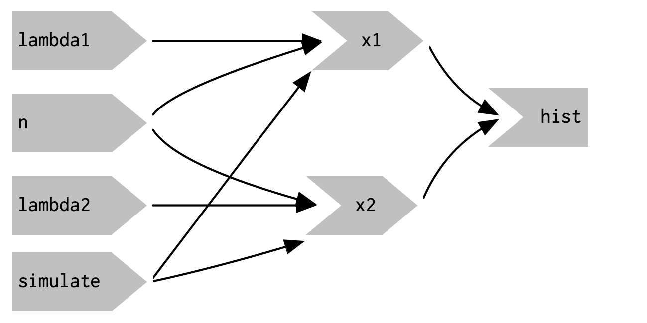{#fig-03-13fig-alt="lambda1 and n connect to x1, lambda2 and n connect to x2. x1 and x2 connect to the hist output. Additionally there is another input from the action button that connects also to x1 and x2." fig-align="center"width="70%"}::: {.my-code-collection}:::: {.my-code-collection-header}::::: {.my-code-collection-icon}::::::::::: {#exm-03-compare-simulated-data6-action-button2}: Case study: Compare simulated data V6 (action button V2)::::::::::::::{.my-code-collection-container}::: {.panel-tabset}###### Code:::::{.my-r-code}:::{.my-r-code-header}:::::: {#cnj-03-compare-simulated-data-code6-action-button2}: Case study: Compare simulated data V6 (action button V2):::::::::::::{.my-r-code-container}::: {#lst-03-compare-simulated-data-code6-action-button2}```{r}#| label: compare-simulated-data-code6-action-button2#| eval: false# source .R file with the two functions didn't workbase::source(base::paste0(here::here(),"/R/shiny-03-V2.R"),local=TRUE,chdir = TRUE,encoding = "utf-8")library(shiny)library(ggplot2)library(munsell)ui<- fluidPage(fluidRow(column(3,numericInput("lambda1", label = "lambda1", value = 3),numericInput("lambda2", label = "lambda2", value = 5),numericInput("n", label = "n", value = 1e4, min = 0),actionButton("simulate","Simulate!")),column(9, plotOutput("hist"))))server<- function(input, output, session){x1<- eventReactive(input$simulate, {rpois(input$n, input$lambda1)})x2<- eventReactive(input$simulate, {rpois(input$n, input$lambda2)})output$hist<- renderPlot({freqpoly(x1(), x2(), binwidth = 1, xlim = c(0, 40))}, res = 96)}shinyApp(ui, server)```Action button to compare a frequency polygon of random numbers drawn from two Poisson distributions (Version 2).:::Compare this code with the wrong V1 version in @lst-03-compare-simulated-data-code5-action-button1.:::::::::###### Shiny:::::{.my-r-code}:::{.my-r-code-header}:::::: {#cnj-03-compare-simulated-data-shiny6-action-button2}: Case study: Compare simulated data V6 (action button V2):::::::::::::{.my-r-code-container}```{shinylive-r}#| standalone: true#| viewerHeight: 600# source .R file with the two functions didn't workfreqpoly<- function(x1, x2, binwidth = 0.1, xlim = c(-3, 3)){df<- base::data.frame(x = base::c(x1, x2),g = base::c(base::rep("x1", base::length(x1)),base::rep("x2", base::length(x2))))ggplot2::ggplot(df, ggplot2::aes(x, colour = g))+ggplot2::geom_freqpoly(binwidth = binwidth, linewidth = 1)+ggplot2::coord_cartesian(xlim = xlim)}t_test<- function(x1, x2){test<- stats::t.test(x1, x2)# use sprintf() to format t.test() results compactlybase::sprintf("p value: %0.3f\n[%0.2f, %0.2f]",test$p.value, test$conf.int[1], test$conf.int[2])}# source(# paste0(here::here(), "/R/shiny-03-V2.R"),# local = TRUE,# chdir = TRUE,# encoding = "utf-8"# )library(shiny)library(ggplot2)library(munsell)ui<- fluidPage(fluidRow(column(3,numericInput("lambda1", label = "lambda1", value = 3),numericInput("lambda2", label = "lambda2", value = 5),numericInput("n", label = "n", value = 1e4, min = 0),actionButton("simulate","Simulate!")),column(9, plotOutput("hist"))))server<- function(input, output, session){x1<- eventReactive(input$simulate, {rpois(input$n, input$lambda1)})x2<- eventReactive(input$simulate, {rpois(input$n, input$lambda2)})output$hist<- renderPlot({freqpoly(x1(), x2(), binwidth = 1, xlim = c(0, 40))}, res = 96)}shinyApp(ui, server)```:::::::::Press the "Simulate" button to compare another step of the two Poison distribution. Observe that changes in the input field does not start the calculation and redrawing of the graph.Compare the code in @lst-03-compare-simulated-data-code6-action-button2 for this shiny app.::::::::::::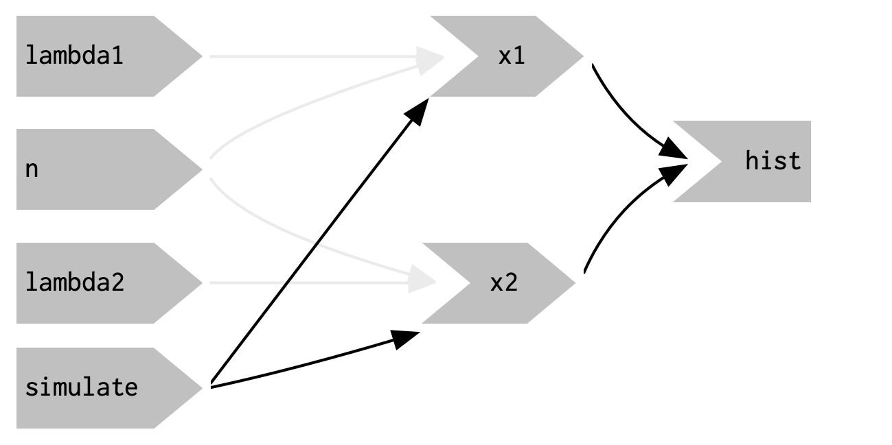{#fig-03-14fig-alt="x1 and x2 no longer have a reactive dependency on (are connected to) lambda1, lambda2, and n. There arrows in pale grey that show the connection of lambda1 and n to x1 as well the connection of lambda2 and n to x2. These pale grey arrows will remind you that x1 and x2 continue to use the values, but no longer take a reactive dependency on them." fig-align="center" width="50%"}## Observers {#sec-03-observers}So far, we’ve focused on what’s happening inside the app. But sometimes you need to reach outside of the app and cause side-effects to happen elsewhere in the world. This might be saving a file to a shared network drive, sending data to a web API, updating a database, or (most commonly)printing a debugging message to the console. These actions don’t affect how your app looks, so you shouldn’t use an output and a render function. Instead you need to use an `r glossary("observer")`.There are multiple ways to create an observer, and we’ll come back to them later in @sec-15-observers-and-outputs. For now, I wanted to show you how to use `shiny::observeEvent()`, because it gives you an important debugging tool when you’re first learning Shiny.`shiny::observeEvent()`is very similar to `shiny::eventReactive()`. It has two important arguments: `eventExpr`and`handlerExpr`.-`eventExpr`is the input or expression to take a dependency on.-`handlerExpr`is the code that will be run. For example, the following modification to `shiny::server()`means that every time that name is updated, a message will be sent to the console.::: {.my-code-collection}:::: {.my-code-collection-header}::::: {.my-code-collection-icon}::::::::::: {#exm-03-message-when-input-updated}: Message whenever the input is updated::::::::::::::{.my-code-collection-container}::: {.panel-tabset}###### Code:::::{.my-r-code}:::{.my-r-code-header}:::::: {#cnj-03-message-when-input-updated-code}: Message whenever the input is updated:::::::::::::{.my-r-code-container}::: {#lst-03-message-when-input-updated-code}```{r}#| label: message-when-input-updated-code#| eval: falselibrary(shiny)ui<- fluidPage(textInput("name","What's your name?"),textOutput("greeting"))server<- function(input, output, session){string<- reactive(paste0("Hello ", input$name, "!"))output$greeting<- renderText(string())observeEvent(input$name, {message("Greeting performed")})}shinyApp(ui, server)```Example of using `shiny::observeEvent`::::::::::::###### Shiny:::::{.my-r-code}:::{.my-r-code-header}:::::: {#cnj-03-message-when-input-updated-shiny}: Message whenever the input is updated:::::::::::::{.my-r-code-container}```{shinylive-r}#| standalone: truelibrary(shiny)ui<- fluidPage(textInput("name","What's your name?"),textOutput("greeting"))server<- function(input, output, session){string<- reactive(paste0("Hello ", input$name, "!"))output$greeting<- renderText(string())observeEvent(input$name, {message("Greeting performed")})}shinyApp(ui, server)```***Look at @lst-03-message-when-input-updated-code the code for this app.::: {.callout-warning}`shiny::observeEvent()`does work as a separate app, but does not work with {**shinylive**}, e.g. it does not send a message neither to the console nor to the HTML web page. I assume it has again to do with variable scoping rules or with the {**shinylive**} configuration.::::::::::::::::::::::::There are two important differences between `shiny::observeEvent()`and`shiny::eventReactive()`:- You don’t assign the result of `observeEvent()`to a variable, so- You can’t refer to it from other reactive consumers.Observers and outputs are closely related. You can think of outputs as having a special side-effect: updating the HTML in the user’s browser. To emphasize this closeness, we’ll draw them the same way in the reactive graph. This yields the following reactive graph shown in @fig-03-15.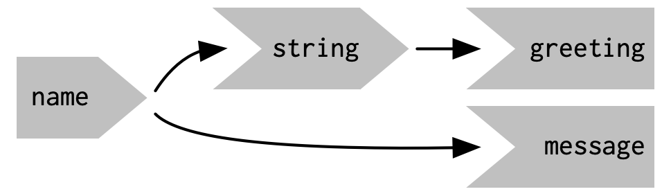{#fig-03-15fig-alt="The input 'name' is connected to 'string' and to the output 'message'. The 'string' element is connected to the output 'greeting'." fig-align="center"width="40%"}## Summary::: {.callout-note}This is already my third reading of this chapter. Each reading lies about one year apart.The first and second time I thought that each example is easy to understand and that the chapter as a whole is straightforward. But it turned out that I was wrong!As a summary I will I will again read the text. But this time I will pay attention to each line of code and write down every tiny example. Additionally I will create my own example and / or invoke the debugger to experiment with the code to understand exactly what is happening inside the server part.:::### Minimal exampleA minimal example consists of four lines of code:::: {.column-body-outset}:::::{.my-r-code}:::{.my-r-code-header}:::::: {#cnj-03-summary-minimal-example}: Minimal example:::::::::::::{.my-r-code-container}::: {#lst-03-summary-minimal-example}```{shinylive-r}#| standalone: true#| components: [editor, viewer]library(shiny)ui<- fluidPage()server<- function(input, output, session){}shinyApp(ui, server)```Minimal example:::::::::::::::There is no error if you run this code. But there is no output as well! The result is an empty white pane.### Printing messages from ui and server partThe problem in my understanding became obvious, when I tried to display just one text message inside the `ui()`and the other one from inside the `server()`function. To make my difficulties explicit I will separate the task in several steps.::: {.column-body-outset}:::::{.my-experiment}:::{.my-experiment-header}:::::: {#def-03-summary-print-ui-server-messages}: Printing messages from ui and server part:::::::::::::{.my-experiment-container}::: {.panel-tabset}###### comments:::::{.my-r-code}:::{.my-r-code-header}:::::: {#cnj-03-summary-comments}: Minimal example with comments in the code:::::::::::::{.my-r-code-container}```{shinylive-r}#| standalone: true#| components: [editor, viewer]library(shiny)ui<- fluidPage(# front end interface)server<- function(input, output, session){# back end logic}shinyApp(ui, server)```:::::::::###### print statements:::::{.my-r-code}:::{.my-r-code-header}:::::: {#cnj-03-summary-print-statements}: Minimal example with print statements in UI and server function:::::::::::::{.my-r-code-container}::: {#lst-03-summary-print-statements}```{shinylive-r}#| standalone: true#| components: [editor, viewer]library(shiny)ui<- fluidPage(print("front end interface"))server<- function(input, output, session){print("back end logic")}shinyApp(ui, server)```Trying to print statements from inside UI and server:::***As you can see only the print statement from the UI is visible. The app does not produce an error and it even produces an output from the server function to the console. But the server print statement does not appear inside the app.:::::::::Compare this failed experiment wit the correct solution in @lst-03-summary-reactive-context. ###### reactive context::: {#lst-03-summary-reactive-context}```{shinylive-r}#| standalone: true#| components: [editor, viewer]library(shiny)ui<- fluidPage(print("front end interface"),textOutput("my_msg"))server<- function(input, output, session){output$my_msg<- renderText("back end logic")}shinyApp(ui, server)```To print statements that appear inside the app you need to provide a `r glossary("reactive context")`.::::::::::::::::::### Failed approachesI will now list several approaches that will fail with their error messages. I hope that this would be helpful to understand better the effect of the reactive context.But I have to fake the error messages as with the `shinylive`extension Shiny will either only produce an empty white pane or display a different error message. I create therefore external Shiny apps, run them with the wrong code snippets and copy the generated error message in this Quarto document.::: {.column-body-outset}:::::{.my-experiment}:::{.my-experiment-header}:::::: {#def-03-summary-failed-approaches}: Why several other approaches will fail?:::::::::::::{.my-experiment-container}::: {.panel-tabset}###### input error 1:::::{.my-r-code}:::{.my-r-code-header}:::::: {#cnj-03-summary-input-error}: Assigning values to input objects inside the server function is not allowed:::::::::::::{.my-r-code-container}::: {#lst-03-summary-input-error-1}```{shinylive-r}#| standalone: true#| components: [editor, viewer]library(shiny)ui<- fluidPage(textInput("msg","front end interface"))server<- function(input, output, server){input$msg<- "back end logic"}shinyApp(ui, server)````input`objects are read-only.:::***> Error in`$<-`(`*tmp*`, msg, value = "back end logic"):> Can't modify read-only reactive value 'msg':::::::::The `input` argument is a list-like object, but unlike a typical list, `input` objects are read-only. If you attempt to modify an input inside the server function, you’ll get the above error.::: {.callout-note}This error occurs because input reflects what’s happening in the browser, and the browser is Shiny’s “single source of truth”. If you could modify the value in R, you could introduce inconsistencies, where the input text said one thing in the browser, and `input$msg` said something different in R. That would make programming challenging! Later, in @sec-chap08, you’ll learn how to use functions like `updateTextInput()` to modify the value in the browser, and then `input$msg` will update accordingly.:::###### input error 2:::::{.my-r-code}:::{.my-r-code-header}:::::: {#cnj-03-summary-input-error-2}: Reading from `input` needs a reactive context:::::::::::::{.my-r-code-container}::: {#lst-03-summary-input-error-2} ```{shinylive-r}#| standalone: true#| components: [editor, viewer]library(shiny)ui <- fluidPage( textInput("msg", "back end logic" ))server <- function(input, output, server) { message("This is the ", input$msg)}shinyApp(ui, server)```To read from an input, you must be in a reactive context.:::***> Error in input$msg : > Can't access reactive value 'msg' outside of reactive consumer. > ℹ Do you need to wrap inside reactive()or observe()?:::::::::`input`is selective about who is allowed to read it. To read from an input, you must be in a reactive context created by a function like `renderText()`or`reactive()`. This is an important constraint that allows outputs to automatically update when an input changes.###### output error 1:::::{.my-r-code}:::{.my-r-code-header}:::::: {#cnj-03-summary-output-error-1}:`output`needs a render function:::::::::::::{.my-r-code-container}::: {#lst-03-summary-output-error-1}```{shinylive-r}#| standalone: true#| components: [editor, viewer]library(shiny)ui<- fluidPage(textOutput("msg"))server<- function(input, output, server){output$msg<- "back end logic"}shinyApp(ui, server)````output`needs a reactive context, it has to be inside a render function.:::***> Error in`.subset2(x,"impl")$defineOutput(name, value, label)`:> Unexpected character object for output$msg> ℹ Did you forget to use a render function?:::::::::Forgetting to put the `output`inside a render function results in the above error.###### output error 2:::::{.my-r-code}:::{.my-r-code-header}:::::: {#cnj-03-summary-output-error-2}:`output`needs a render function:::::::::::::{.my-r-code-container}::: {#lst-03-summary-output-error-2}```{shinylive-r}#| standalone: true#| components: [editor, viewer]library(shiny)ui<- fluidPage(textOutput("msg"))server<- function(input, output, server){message("This is the ", output$msg)}shinyApp(ui, server)```You can't read from `output` outside a reactive context.:::***> Error in `output$msg` : Can't read output 'msg':::::::::Reading from the `output`is not allowed:::::::::::::::### Reactivity templateThe most elemental shiny app has just one `r glossary("reactive context")`. It consists of one `output`that is automatically updated whenever its only `input`changes.The next example implements this minimal reactivity in Shiny. ::: {.column-body-outset}:::::{.my-r-code}:::{.my-r-code-header}:::::: {#cnj-03-summary-reactivity-template}: Five parts of a reactive context:::::::::::::{.my-r-code-container}::: {#lst-03-summary-reactivity-template}```{shinylive-r}#| standalone: true#| components: [editor, viewer]ui<- fluidPage(textInput("name","What's your name?"),textOutput("greeting"))server<- function(input, output, session){output$greeting<- renderText({paste0("Hello ", input$name, "!")})}shinyApp(ui, server)```Five parts of a reactive context :::::::::::::::The above code works for me as a kind of mental device that helps me to remember the five parts of a reactive context:1.**Input in the UI function**, so that user can provide whatever input they want (but restricted to the list of Shiny input categories.)2.**Output in the UI function**, so that the provided input can be transferred to the server logic.3.**Input in the server function** with the fixed pattern `input$<inputID>`where`inputID`works as a reference to the front end.4.**Output in the server function** with the pattern `output$<outputID>`where`outputID`is a reference to the front end type of output.5.**Reactive function** appropriate for the output type which assigns /connect the `input$<inputID>`to the `output$<outputID>`.or in a more general form:1.`<type>Input`with`<type>InputID`(UI)2.`<type>Output`with`<type>OutputID`(UI)3.`input$<inputID>`(server)4.`output$<outputID>`(server)5. reactive function### Reactive expressions#### Basic principle:::::{.my-r-code}:::{.my-r-code-header}:::::: {#cnj-03-summary-reactive-expression}: Reactive Expression:::::::::::::{.my-r-code-container}```{shinylive-r}#| standalone: true#| components: [editor, viewer]library(shiny)ui<- fluidPage(textInput("name","What's your name?"),textOutput("greeting"))server<- function(input, output, session){string<- reactive(paste0("Hello ", input$name, "!"))output$greeting<- renderText(string())}shinyApp(ui, server)```***Compare the code with @lst-03-summary-reactivity-template.:::::::::The important point of `r glossary("reactive expressions")`is that they mediate between `input`and`output`.`string`works as an mediator between `input$name`and`output$greeting`.We can think of reactive expressions as tools to reduces duplication in the reactive code by introducing additional nodes into the `r glossary("reactive graph")`. Te reactive expression can be used like a function and like a function it is called with `()`at the end of its name. But it never has arguments between its parenthesis. #### Practical exampleIn the case above we didn't use the additional node, to simplify the code. In order to understand why we need `r glossary("reactive epxressions")` we need a more complex example. Hadley offers in the book the comparison of two simulated datasets with a plot and a hypothesis test. I am planning to generate a simpler example. STILL TO DO -> @XXX_practical-example```{r}#| label: practical-example#| eval: false#| include: falsex <- round(rnorm(10000, mean = 0, sd = 1), 2)y <- round(runif(10000, min = 1, max = 100), 0)df <- data.frame(x, y)ggplot2::ggplot(df, ggplot2::aes(x)) + ggplot2::geom_histogram(bins = 30)```## Glossary Entries {#unnumbered}```{r}#| label: glossary-table#| echo: falseglossary_table()```------------------------------------------------------------------------## Session Info {.unnumbered}::: my-r-code::: my-r-code-headerSession Info:::::: my-r-code-container```{r}#| label: session-infosessioninfo::session_info()```::::::


