If you’re going to be writing a lot of Shiny apps (and since you’re reading this book I hope you will be!), it’s worth investing some time in your basic workflow. Improving workflow is a good place to invest time because it tends to pay great dividends in the long run. It doesn’t just increase the proportion of your time spent writing R code, but because you see the results more quickly, it makes the process of writing Shiny apps more enjoyable, and helps your skills improve more quickly.
Objectives of chapter on Workflow
The goal of this chapter is to help you improve three important Shiny workflows:
The basic development cycle of creating apps, making changes, and experimenting with the results.
Debugging, the workflow where you figure out what’s gone wrong with your code and then brainstorm solutions to fix it.
Writing reprexes, self-contained chunks of code that illustrate a problem. Reprexes are a powerful debugging technique, and they are essential if you want to get help from someone else.
5.1 Development workflow
There are two main workflows to optimize here:
creating an app for the first time, and
speeding up the iterative cycle of tweaking code and trying out the results.
5.1.1 Creating the app
5.1.1.1 Code snippets
Every app starts with the same six lines of R code. (The repetitive usage of code is not only for Shiny important. I have developed a huge amount of code snippets for R and even more for Markdown). For instance all the (code) boxes (e.g., Resource 5.1) you see in my notes are created by inserting templates via code snippets. In the next paragraph I will type at the beginning of the line num-resources and with SHIFT-TAB my template for a numbered resource box is created. I just have to add IDs for generating internal links and the content.
:::::{.my-resource}:::{.my-resource-header}:::::: {#lem-resource-text}: Numbered Resource Title:::::::::::::{.my-resource-container}Here include text for the resource:::::::::
If you want to start a new project, go to the File menu, select “New Project” then select “Shiny Web Application”.
5.1.1.3 New Shiny app in existing project
Here I am using my “learning-shiny” book project to develop several shiny apps. Go to the File menu, select “New File”->“Shiny Web App…”. This opens up a window to name a folder where the app.R file for the Shiny app is created. The name of the folder is essential as all Shiny apps have the same file name (app.R) if you choose (as I do) a single file app.
Picture 5.1: Window for creating a new shiny app inside a project
5.1.1.4 New shinylive code chunk
Here in this book I am predominantly using the {shinylive} package. Therefore I have prepared another markdown snippet.
I knew about the shortcut CMD-SHIFT-ENTER for running the current code chunk. I didn’t know that the same shortcut could be used for the shiny app. But it is a sensible generalization. What else is a shiny app as one (big) code chunk?
I didn’t know nothing about background jobs except that it is invoked by rendering the Quarto file. Actually I don’t know if it is still necessary to invoke the procedure described in Shiny apps in background jobs. The reason is that Shiny will run in the background if I enter the shortcut CMD-SHIFT-ENTER inside the Shiny app script.
There is some small change about the workflow as described in the section “Seeing your changes” in chapter 5 of the website of the Mastering Shiny book. Instead of “Write some code and press Cmd/Ctrl + S to save the file.” it works for me with “Write some code and press Cmd/Ctrl-Shift-Enter to save and run the reloaded changed file.”
Procedure 5.1 : Shiny background job
Write some code and press Cmd/Ctrl-Shift-Enter.
Interactively experiment.
Go to 1.
The chief disadvantage of this technique is that it’s considerably harder to debug because the app is running in a separate process.
But the general procedure to start background jobs inside the RStudio environment is very valuable for me. I could use background workflows with lengthy rendering procedures of my Quarto note books.
To call the procedure in Procedure 5.1 you have to tick the option “In Background Job” in the “Run App”-button (see Picture 5.2). (You see this window only in inside the script of the Shiny app.)
Run in Window open the app in a pop-out RStudio window. This has the interesting side effect, that it always open an new tab if the Shiny app is run again. This is nice for comparing different version. If you have a second screen you can move the window out of the code view and display both app code and app result at the same time.
Run in Viewer Pane opens the app in the RStudio viewer pane (usually located on the right hand (bottom) side of the IDE. It’s useful for smaller apps because you can see it at the same time as you run your app code.
Run External” opens the app in your usual web browser. It’s useful for larger apps and when you want to see what your app looks like in the context that most users will experience it. Again you can look at both (Code and running app)at the same time with a second display. (But I prefer the large main screen changing between RStudio and browser with shortcuts.)
Picture 5.2: The run app button allows you to choose if the app runs in the console or as background job and how the running app will be shown
With an external browser window there are is one observation I made: If you shut down the background job or restart R then the browser window is invalidated and running the app again will open a new tab in your browser. This is contrast to rendering a Quarto document showing in an external browser window. Closing this window will not show the new results in a new browser window. You have to restart R, then RStudio will open a new browser window after the rendering process is finished.
5.2 Debugging
There are three main cases of problems which we’ll discuss below:
Unexpected error: This is the easiest case, because you’ll get a traceback which allows you to figure out exactly where the error occurred. Once you’ve identified the problem, you’ll need to systematically test your assumptions until you find a difference between your expectations and reality. The interactive debugger is a powerful assistant for this process.
Incorrect value: You don’t get any errors, but some value is incorrect. Here, you’ll need to use the interactive debugger, along with your investigative skills to track down the root cause.
Shiny does not update correctly: All the values are correct, but they’re not updated when you expect. This is the most challenging problem because it’s unique to Shiny, so you can’t take advantage of your existing R debugging skills.
5.2.1 Talk by Jenny Brian
I am relatively unexperienced with R debugging. So I started with the Jenny Bryan’s talk. What follows is short summary of the talk:
Procedure 5.2 : General debugging procedures following the Jenny Brian video lecture
There are three general procedures:
Restart R very often and if it stuck restart RStudio. As a last resort you could also start your computer. This cleans all hanging cached variables or hanging processes. (This process I have already standard behavior for me.)
Reprex: Learn how to communicate for help with minimalreprexes. I am already used reprexes. It is a challenge but very useful, sometimes I have solved the problem on my own during the process of creating a minmal reprex.
Debugging: There are three different general aspects:
back::traceback(), last_trace::rlang() is like reading a death certificate. back::traceback() is to be read from bottom to top; last_trace::rlang() is easier to read from top to bottom and has a nested view.
base::options(error = utils::recover): This is like a post-mortem autopsy. This function allows the user to browse directly on any of the currently active function calls, and is suitable as an error option. When called, recover prints the list of current calls, and prompts the user to select one of them. The standard R browser is then invoked from the corresponding environment; the user can type ordinary R language expressions to be evaluated in that environment such as: utils::ls.str().
base::browser() statement (or in RStudio a break point) written into the appropriate place of the code, general at the start of a function. This is like a reanimation. Stopping debugging with Q (Alternatives are base::debug() with base::undebug(), base::debugonce() or in RStudio choose Stop Debugging from the Debug menu or type the shortcut Shift-F8).
RStudio has a very handy starting debugging feature where you choose to hide the traceback or to rerun it with debug.
Picture 5.3: RStudio debugging feature: Slide from Jenny Brian’s video talk
Tip 5.1: Deter next error
As debugging is intimidating Jenny Bryan recommends at the end of her talk three debugging learning strategies:
Reserve a time box for debugging (e.g. 10-15 min) for the next error I can’t find immediately. If you haven’t resolved the issue return back to your used procedures. (This is easy to apply and I will try it the next time.)
Prepare for the unexpected future by using the {testthat} package. It supports a testing framework for R that integrates with your existing ‘workflow’.
Only the first tip is at the moment for me easy to apply. Of the other three strategies I have already heard, but they are at the moment in my daily work behavior with R difficult to include. I will try them out when I return to develop an R package for general use.
5.2.2 Tracebacks in Shiny
You can’t use traceback() in Shiny because you can’t run code while an app is running. Instead, Shiny will automatically print the traceback for you.
R Code 5.1 : Example: Traceback in {shiny}
Listing / Output 5.1: An example of Shiny traceback
The following error message is faked (copied from a live shiny app), because it does not work with {shinylive}. {shinylive} produces just the same message as inside the app:
Error: non-numeric argument to binary operator
Warning: Error in *: non-numeric argument to binary operator
  178: g […/app.R#4]
  177: f […/app.R#3]
  176: renderPlot […/app.R#13]
  174: func
  134: drawPlot
  120: <reactive:plotObj>
  100: drawReactive
   87: renderFunc
   86: output$plot
    1: shiny::runApp
I have the first three line edited so that they do not reveal my internal directory organisation.
To understand what’s going on we again start by flipping it upside down, so you can see the sequence of calls in the order they appear:
Starting the app: The first few calls start the app. In this case, you just see shiny::runApp(), but depending on how you start the app, you might see something more complicated. For example, if you called base::source() to run the app, you might see this:
1: source3: print.shiny.appobj5: runApp
In general, you can ignore anything before the first runApp(); this is just the setup code to get the app running.
Reactive expression: Next, you’ll see some internal Shiny code in charge of calling the reactive expression:
Here, spotting output$plot is really important — that tells which of your reactives (plot) is causing the error. The next few functions are internal, and you can ignore them.
Actual code: Finally, at the very bottom, you’ll see the code that you have written:
  176: renderPlot […/app.R#13]
  177: f […/app.R#3]
  178: g […/app.R#4]
This is the code called inside of renderPlot(). You can tell you should pay attention here because of the file path and line number; this lets you know that it’s your code.
Watch out!
If you get an error in your app but don’t see a traceback then make sure that you’re running the app using Cmd/Ctrl + Shift + Enter (or if not in RStudio, calling runApp()), and that you’ve saved the file that you’re running it from. Other ways of running the app don’t always capture the information necessary to make a traceback.
5.2.3 The interactive debugger
Once you’ve located the source of the error and want to figure out what’s causing it, the most powerful tool you have at your disposal is the interactive debugger. The debugger pauses execution and gives you an interactive R console where you can run any code to figure out what’s gone wrong. There are two ways to launch the debugger:
browser() function call: Add a call to base::browser() in your source code. This is the standard R way of launching the interactive debugger, and will work however you’re running Shiny. The advantage of browser() is that because it’s R code, you can make it conditional by combining it with an if statement. This allows you to launch the debugger only for problematic inputs.
if (input$value == "a") { browser()}# Or maybeif (my_reactive() < 0) { browser()}
RStudio breakpoint: Add an RStudio breakpoint by clicking to the left of the line number. You can remove the breakpoint by clicking on the red circle. The advantage of breakpoints is that they’re not code, so you never have to worry about accidentally checking them into your version control system.
Picture 5.4: Setting a breakpoint in RStudio
If you’re using RStudio, the toolbar in Picture 5.5 will appear at the top of the console when you’re in the debugger. The toolbar is an easy way to remember the debugging commands that are now available to you. They’re also available outside of RStudio; you’ll just need to remember the one letter command to activate them. The three most useful commands are:
Next (press n): executes the next step in the function. Note that if you have a variable named n, you’ll need to use print(n) to display its value.
Continue (press c): leaves interactive debugging and continues regular execution of the function. This is useful if you’ve fixed the bad state and want to check that the function proceeds correctly.
Stop (press Q): stops debugging, terminates the function, and returns to the global workspace. Use this once you’ve figured out where the problem is, and you’re ready to fix it and reload the code.
Picture 5.5: RStudio’s debugging scenario: Waiting at the breakpoint, involing the debugger
As well as stepping through the code line-by-line using these tools, you’ll also write and run a bunch of interactive code to track down what’s going wrong. Debugging is the process of systematically comparing your expectations to reality until you find the mismatch. If you’re new to debugging in R, you might want to read the Debugging chapter of “Advanced R” to learn some general techniques.
Resource 5.3 : Debugging
I have collected some resources for interactive debugging in R.
Hadley Wickham: General advise and problem-solving strategies in Debugging (Chapter 22 in the second edition of the Advanced R book).
The {rlang} package is a collection of frameworks and APIs for programming with R. (I’ve already learned about this package, but it seems that it is — at least at the moment, June 2025 — a resource for more experienced programmers than me.)
5.2.4 Case study
I skip over the interesting and illuminating case study because reproducing the reported strategies is not educationally valuable. I would need my own problem to debug.
Important
In the case study there are two important learnings for me:
Assuming some line of code is the trouble maker try to reproduce the problem in the console outside the debugger!
Inside the debugger try the interactive console to verify if you are in problematic line of code!
By the way: I ran over a similar problem as reported in the case study. Instead of confusing “NA” for North America with NA I had the ISO 3166 two letter country code (alpha2) with “NA”. (See filteredc dataset to “Namibia” in opendatasoft)
5.2.5 Debugging reactivity
The hardest type of problem to debug is when your reactives fire in an unexpected order. At this point in the book, we have relatively few tools to recommend to help you debug this issue. In the next section, you’ll learn how to create a minimal reprex which is crucial for this type of problem, and later in the book, you’ll learn more about the underlying theory, and about tools like the reactivity visualizer {reactlog} (Schloerke 2022). But for now, we’ll focus on a classic technique that’s useful here: “print” debugging.
The basic idea of print debugging is to call print() whenever you need to understand when a part of your code is evaluated, and to show the values of important variables. We call this “print” debugging (because in most languages you’d use a print function), but In R it makes more sense to use message():
base::print() is designed for displaying vectors of data so it puts quotes around strings and starts the first line with “[1]”.
base::message() sends its result to “standard error”, rather than “standard output”. These are technical terms describing output streams, which you don’t normally notice because they’re both displayed in the same way when running interactively. But if your app is hosted elsewhere, then output sent to “standard error” will be recorded in the logs.
I also recommend coupling message() with the glue() function from the {glue} package, which makes it easy to interleave text and values in a message.2
A final useful tool is utils::str(), which prints the detailed structure of any object. This is particularly useful if you need to double check you have the type of object that you expect.
Summarized there are three tools for print debugging at this state of the notes:
Here’s a toy app that shows off some of the basic ideas. Note how I use message() inside a reactive(): I have to perform the computation, send the message, and then return the previously computed value.
Code Collection 5.1 : Toy example with print debugging
I can’t demonstrate printing the output inside a reactive code snippet with {shinylive} here. Only the output in the not reactive output$total will appear. So I faked the output with copy and paste from the online book:
Updating y from 2 to 2New total is 6
And if I drag the x slider to 3 I see
Updating y from 2 to 6New total is 8New total is 12
Don’t worry if you find the results a little surprising.
Note
Yes, in fact, this is surprising for me, as I get the new total twice! I’ll will wait to learn more about what’s going on in Chapter 8 with the help of the reactive graph diagrams mentioned in Section 3.3.3.
In the meanwhile I have in the next tab changed text and place of the messages in this toy example.
R Code 5.3 : Toy example with my own print debugging messages
The printing command in the total reactive is easier to understand for me. But I think the places for the message() command in the book example are on those other places to show an specific behavior of the reactivity behavior of this Shiny toy example.
> shiny::runApp('apps-05/print-debugging')Loading required package: shinyListening on http://127.0.0.1:7653# After started the appNew total is x+y+z = 1 + 2 + 3 = 6# After dragging the x slider to 3New total is x+y+z = 3 + 2 + 3 = 8New total is x+y+z = 3 + 6 + 3 = 12
5.3 Getting help
I will shorten this section as I have already some experiences with reprexes. I will focus on those points that are not so obvious for me.
5.3.1 Reprex basics
{reprex} package: In the book the usage of the {reprex} package is not mentioned. It is a very useful tool and simplifies the technical process of catching the code. I am using the {reprex} package (Bryan et al. 2024) with RStudio addins, because that makes it much comfortable to use.
5.3.2 Making a reprex
This section does not mention the technical process but focuses on conceptional issues.
Typically, the most challenging part of making your app work on someone else’s computer is eliminating the use of data that’s only stored on your computer. There are four useful patterns:
5.3.2.1 Built-in datset
Often the data you’re using is not directly related to the problem, and you can instead use a built-in dataset like mtcars or iris.
5.3.2.2 R Code dataset
Other times, you might be able to write a little R code that creates a dataset that illustrates the problem:
Code
mydata<-data.frame(x =1:5, y =c("a", "b", "c", "d", "e"))mydata
#>   x y
#> 1 1 a
#> 2 2 b
#> 3 3 c
#> 4 4 d
#> 5 5 e
5.3.2.3dput() dataset
If both of those techniques fail, you can turn your data into code with base::dput(). For example, dput(mydata) generates the code that will recreate `mydata```:
#> structure(list(x = 1:5, y = c("a", "b", "c", "d", "e")), class = "data.frame", row.names = c(NA,
#> -5L))
Once you have that code, you can put this in your reprex to generate mydata:
Code
mydata<-structure(list(x =1:5, y =structure(1:5, .Label =c("a", "b","c", "d", "e"), class ="factor")), class ="data.frame", row.names =c(NA,-5L))mydata
#>   x y
#> 1 1 a
#> 2 2 b
#> 3 3 c
#> 4 4 d
#> 5 5 e
Often, running dput() on your original data will generate a huge amount of code, so find a subset of your data that illustrates the problem. The smaller the dataset that you supply, the easier it will be for others to help you with your problem.
5.3.2.4 Complete project
If reading data from disk seems to be an irreducible part of the problem, a strategy of last resort is to provide a complete project containing both an app.R and the needed data files. The best way to provide this is as a RStudio project hosted on GitHub, but failing that, you can carefully make a zip file that can be run locally.
Make sure that you use relative paths (i.e. read.csv("my-data.csv") not read.csv("c:\\my-user-name\\files\\my-data.csv")) so that your code still works when run on a different computer.
You should also consider the reader and spend some time formatting your code so that it’s easy to read. If you adopt the tidyverse style guide, you can automatically reformat your code using the {styler} package; that quickly gets your code to a place that’s easier to read.
5.3.3 Making a minimal reprex
Creating the smallest possible reprex is particularly important for Shiny apps, which are often complicated. But — as Jenny Bryan mentioned in her talk (see Section 5.2.1) — creating a minimal reprex is both a science and an art.
Tip 5.2: Debugging strategy but also a way to make a minimal reprex
If you don’t know what part of your code is triggering the problem, a good way to find it is to remove sections of code from your application, piece by piece, until the problem goes away.
Alternatively, sometimes it’s simpler to start with a fresh, empty, app and progressively build it up until you find the problem once more.
Checklist 5.1
: Take a final pass through your Reprex
Is every input and output in UI related to the problem?
Does your app have a complex layout that you can simplify to help focus on the problem at hand? Have you removed all UI customisation that makes your app look good, but isn’t related to the problem?
Are there any reactives in server() that you can now remove?
If you’ve tried multiple ways to solve the problem, have you removed all the vestiges of the attempts that didn’t work?
Is every package that you load needed to illustrate the problem? Can you eliminate packages by replacing functions with dummy code?
5.3.4 Case Study
Again I will skip the case study, especially as I can’t demonstrate it with a {**shinylive*} chunk. But I have provided the shiny apps in the “app05” folder.
Another remark: I got slightly different error messages. For instance instead of ““Type mismatch for min, max, and value. Each must be Date, POSIXt, or number” in the first case study example I got “Error in min: invalid ‘type’ (list) of argument” with my experiment in the console.
5.4 Summary
This chapter has given you some useful workflows for developing apps, debugging problems, and getting help. These workflows might seem a little abstract and easy to dismiss because they’re not concretely improving an individual app. But I think of workflow as one of my “secret” powers: one of the reasons that I’ve been able to accomplish so much is that I devote time to analysing and improving my workflow. I highly encourage you to do the same!
The next chapter on layouts and themes is the first of a grab bag of useful techniques. There’s no need to read in sequence; feel free to skip ahead to a chapter that you need for a current app.
Note 5.1
I will follow the advice and continue with #sec-chap09 because I need the upload of a dataset for the work on my first real Shiny app.
5.5 Glossary Entries
term
definition
IDEx
An Integrated Development Environment (IDE) is a software application that helps programmers develop software code efficiently. It typically includes features such as a source code editor, build automation tools, and a debugger.
REPREX
Reprex is an REPRoducable EXample. A reprex makes a conversation about code more efficient and pleasant for all. This comes up whenever you ask someone for help, report a bug in software, or propose a new feature. The habit of making little, rigorous, self-contained examples also has the great side effect of making you think more clearly about your programming problems. In R the reprex package (https://reprex.tidyverse.org) makes it especially easy to prepare R code as a reprex, in order to share it on GitHub, StackOverflow etc.
Bryan, Jennifer, Jim Hester, David Robinson, Hadley Wickham, and Christophe Dervieux. 2024. “Reprex: Prepare Reproducible Example Code via the Clipboard.”https://doi.org/10.32614/CRAN.package.reprex.
This is for me an incomprehensibe error message that I have already experienced several times. It helps very much to replace ‘closure’ with ‘function’.↩︎
As I am already comfortable to use glue() I skip the demonstration how to use the {glue} package.↩︎
Source Code
---execute: cache: true---# Workflow {#sec-chap05}```{r}#| label: setup#| results: hold#| include: falsebase::source(file ="R/helper.R")```If you’re going to be writing a lot of Shiny apps (and since you’rereading this book I hope you will be!), it’s worth investing some timein your basic workflow. Improving workflow is a good place to investtime because it tends to pay great dividends in the long run. It doesn’tjust increase the proportion of your time spent writing R code, butbecause you see the results more quickly, it makes the process ofwriting Shiny apps more enjoyable, and helps your skills improve morequickly.:::::: {#obj-chap05}::::: my-objectives::: my-objectives-headerObjectives of chapter on Workflow:::::: my-objectives-containerThe goal of this chapter is to help you improve three important Shinyworkflows:- The basic development cycle of creating apps, making changes, and experimenting with the results.- Debugging, the workflow where you figure out what’s gone wrong with your code and then brainstorm solutions to fix it.- Writing `r glossary("reprex", "reprexes")`, self-contained chunks of code that illustrate a problem. Reprexes are a powerful debugging technique, and they are essential if you want to get help from someone else.::::::::::::::## Development workflowThere are two main workflows to optimize here:- creating an app for the first time, and- speeding up the iterative cycle of tweaking code and trying out the results.### Creating the app#### Code snippetsEvery app starts with the same six lines of R code. (The repetitiveusage of code is not only for Shiny important. I have developed a hugeamount of code snippets for R and even more for Markdown). For instanceall the (code) boxes (e.g., @lem-05-code-snippets) you see in my notesare created by inserting templates via code snippets. In the nextparagraph I will type at the beginning of the line `num-resources` andwith SHIFT-TAB my template for a numbered resource box is created. Ijust have to add IDs for generating internal links and the content.``` markdown:::::{.my-resource}:::{.my-resource-header}:::::: {#lem-resource-text}: Numbered Resource Title:::::::::::::{.my-resource-container}Here include text for the resource:::::::::```:::::: my-resource:::: my-resource-header::: {#lem-05-code-snippets}: Code snippets:::::::::: my-resource-container- [RStudio code snippets](https://support.rstudio.com/hc/en-us/articles/204463668-Code-Snippets)- [Shiny specific snippets](https://github.com/ThinkR-open/shinysnippets) put together by [ThinkR](https://github.com/ThinkR-open).- [{**shinysnippets**}](https://thinkr-open.github.io/shinysnippets/) package [@shinysnippets]:::::::::#### New Shiny projectIf you want to start a new project, go to the File menu, select “NewProject” then select “Shiny Web Application”.#### New Shiny app in existing projectHere I am using my "learning-shiny" book project to develop severalshiny apps. Go to the File menu, select "New File"-\>"Shiny Web App…".This opens up a window to name a folder where the `app.R` file for theShiny app is created. The name of the folder is essential as all Shinyapps have the same file name (`app.R`) if you choose (as I do) a singlefile app.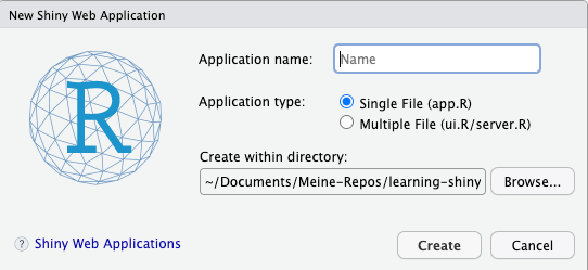{#fig-05-01fig-alt="alt-text" fig-align="center" width="70%"}#### New shinylive code chunkHere in this book I am predominantly using the {**shinylive**} package.Therefore I have prepared another markdown snippet.```` markdown:::{.column-page}:::::{.my-r-code}:::{.my-r-code-header}:::::: {#cnj-ID-text}: Numbered R Code Title:::::::::::::{.my-r-code-container}```{shinylive-r}#| standalone: true#| viewerHeight: 300#| components: [editor, viewer]#| layout: verticallibrary(shiny)start coding here```::::::::::::````### Seeing the changesI knew about the shortcut `CMD-SHIFT-ENTER` for running the current codechunk. I didn't know that the same shortcut could be used for the shinyapp. But it is a sensible generalization. What else is a shiny app asone (big) code chunk?I didn't know nothing about background jobs except that it is invoked byrendering the Quarto file. Actually I don't know if it is stillnecessary to invoke the procedure described in [Shiny apps in backgroundjobs](https://github.com/sol-eng/background-jobs/tree/main/shiny-job).The reason is that Shiny will run in the background if I enter theshortcut CMD-SHIFT-ENTER inside the Shiny app script.There is some small change about the workflow as described in thesection "Seeing your changes" in chapter 5 of the [website of theMastering Shiny book](https://mastering-shiny.org/action-workflow.html).Instead of "Write some code and press Cmd/Ctrl + S to save the file." itworks for me with "Write some code and press Cmd/Ctrl-Shift-Enter tosave and run the reloaded changed file.":::::: my-procedure:::: my-procedure-header::: {#prp-05-shiny-background-job}: Shiny background job:::::::::: my-procedure-container1. Write some code and press Cmd/Ctrl-Shift-Enter.2. Interactively experiment.3. Go to 1.:::::::::The chief disadvantage of this technique is that it’s considerablyharder to debug because the app is running in a separate process.But the general procedure to start background jobs inside the RStudioenvironment is very valuable for me. I could use background workflowswith lengthy rendering procedures of my Quarto note books.:::::: my-resource:::: my-resource-header::: {#lem-05-background-jobs}: Background jobs in the RStudio `r glossary("IDEx", "IDE")`:::::::::: my-resource-container- [Local Job Environment Options](https://github.com/sol-eng/background-jobs/tree/main/shiny-job)- [RStudio Background Jobs](https://posit.co/blog/rstudio-1-2-jobs/):::::::::::: callout-importantTo call the procedure in @prp-05-shiny-background-job you have to tickthe option "In Background Job" in the "Run App"-button (see @fig-05-02).(You see this window only in inside the script of the Shiny app.):::### Controlling the viewThere are three options (see @fig-05-02):1. **Run in Window** open the app in a pop-out RStudio window. This has the interesting side effect, that it always open an new tab if the Shiny app is run again. This is nice for comparing different version. If you have a second screen you can move the window out of the code view and display both app code and app result at the same time.2. **Run in Viewer Pane** opens the app in the RStudio viewer pane (usually located on the right hand (bottom) side of the`r glossary("IDEx", "IDE")`. It’s useful for smaller apps because you can see it at the same time as you run your app code.3. **Run External**" opens the app in your usual web browser. It’s useful for larger apps and when you want to see what your app looks like in the context that most users will experience it. Again you can look at both (Code and running app)at the same time with a second display. (But I prefer the large main screen changing between RStudio and browser with shortcuts.)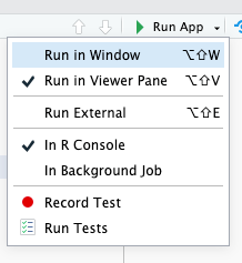{#fig-05-02fig-alt="alt-text" fig-align="center" width="30%"}With an external browser window there are is one observation I made: Ifyou shut down the background job or restart R then the browser window isinvalidated and running the app again will open a new tab in yourbrowser. This is contrast to rendering a Quarto document showing in anexternal browser window. Closing this window will not show the newresults in a new browser window. You have to restart R, then RStudiowill open a new browser window after the rendering process is finished.## DebuggingThere are three main cases of problems which we’ll discuss below:1. **Unexpected error**: This is the easiest case, because you’ll get a traceback which allows you to figure out exactly where the error occurred. Once you’ve identified the problem, you’ll need to systematically test your assumptions until you find a difference between your expectations and reality. The interactive debugger is a powerful assistant for this process.2. **Incorrect value**: You don’t get any errors, but some value is incorrect. Here, you’ll need to use the interactive debugger, along with your investigative skills to track down the root cause.3. **Shiny does not update correctly**: All the values are correct, but they’re not updated when you expect. This is the most challenging problem because it’s unique to Shiny, so you can’t take advantage of your existing R debugging skills.### Talk by Jenny Brian {#sec-05-talk-jeyy-brian}I am relatively unexperienced with R debugging. So I started with theJenny Bryan's talk. What follows is short summary of the talk::::::: my-procedure:::: my-procedure-header::: {#prp-04-debugging}: General debugging procedures following the Jenny Brian video lecture:::::::::: my-procedure-containerThere are three general procedures:1. **Restart R** very often and if it stuck restart RStudio. As a last resort you could also start your computer. This cleans all hanging cached variables or hanging processes. (This process I have already standard behavior for me.)2. **Reprex**: Learn how to communicate for help with *minimal*`r glossary("reprex", "reprexes.")` I am already used reprexes. It is a challenge but very useful, sometimes I have solved the problem on my own during the process of creating a minmal reprex.3. **Debugging**: There are three different general aspects: 1. `back::traceback()`, `last_trace::rlang()` is like reading a death certificate. `back::traceback()` is to be read from bottom to top; `last_trace::rlang()` is easier to read from top to bottom and has a nested view. 2. `base::options(error = utils::recover)`: This is like a post-mortem autopsy. This function allows the user to browse directly on any of the currently active function calls, and is suitable as an error option. When called, recover prints the list of current calls, and prompts the user to select one of them. The standard R browser is then invoked from the corresponding environment; the user can type ordinary R language expressions to be evaluated in that environment such as:`utils::ls.str()`. 3. `base::browser()` statement (or in RStudio a break point) written into the appropriate place of the code, general at the start of a function. This is like a reanimation. Stopping debugging with `Q` (Alternatives are `base::debug()` with`base::undebug()`, `base::debugonce()` or in RStudio choose`Stop Debugging` from the Debug menu or type the shortcut`Shift-F8`).:::::::::RStudio has a very handy starting debugging feature where you choose tohide the traceback or to rerun it with debug.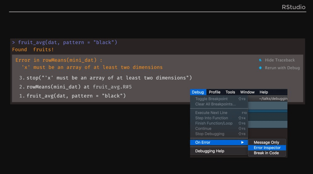{#fig-05-03fig-alt="alt-text" fig-align="center" width="100%"}::: {#tip-05-debugging-jenny-brian .callout-tip}###### Deter next errorAs debugging is intimidating Jenny Bryan recommends at the end of hertalk three debugging learning strategies:1. Reserve a time box for debugging (e.g. 10-15 min) for the next error I can't find immediately. If you haven't resolved the issue return back to your used procedures. (This is easy to apply and I will try it the next time.)2. Prepare for the unexpected future by using the {**testthat**} package. It supports a testing framework for R that integrates with your existing 'workflow'.3. Automate your check with `R CMD` check and `testthat::test_check()`4. Use Github continuous integration:::Only the first tip is at the moment for me easy to apply. Of the otherthree strategies I have already heard, but they are at the moment in mydaily work behavior with R difficult to include. I will try them outwhen I return to develop an R package for general use.### Tracebacks in ShinyYou can’t use traceback() in Shiny because you can’t run code while anapp is running. Instead, Shiny will automatically print the tracebackfor you.::::::: my-r-code:::: my-r-code-header::: {#cnj-05-shiny-traceback}: Example: Traceback in {**shiny**}::::::::::: my-r-code-container::: {#lst-05-shiny-traceback}```{r}#| label: shiny-traceback#| eval: falselibrary(shiny)f <-function(x) g(x)g <-function(x) h(x)h <-function(x) x *2ui <-fluidPage(selectInput("n", "N", 1:10),plotOutput("plot"))server <-function(input, output, session) { output$plot <-renderPlot({ n <-f(input$n)plot(head(cars, n)) }, res =96)}shinyApp(ui, server)```An example of Shiny traceback:::The following error message is faked (copied from a live shiny app),because it does not work with {**shinylive**}. {**shinylive**} producesjust the same message as inside the app:`Error: non-numeric argument to binary operator```` markdownWarning: Error in *: non-numeric argument to binary operator 178: g […/app.R#4] 177: f […/app.R#3] 176: renderPlot […/app.R#13] 174: func 134: drawPlot 120: <reactive:plotObj> 100: drawReactive 87: renderFunc 86: output$plot 1: shiny::runApp```I have the first three line edited so that they do not reveal myinternal directory organisation.:::::::::::To understand what’s going on we again start by flipping it upside down,so you can see the sequence of calls in the order they appear:``` markdown 1: shiny::runApp 86: output$plot 87: renderFunc 100: drawReactive 120: <reactive:plotObj> 134: drawPlot 174: func 176: renderPlot […/app.R#13] 177: f […/app.R#3] 178: g […/app.R#4]```There are three basic parts to the call stack:1. **Starting the app**: The first few calls start the app. In this case, you just see `shiny::runApp()`, but depending on how you start the app, you might see something more complicated. For example, if you called `base::source()` to run the app, you might see this:``` markdown1: source3: print.shiny.appobj5: runApp```In general, you can ignore anything before the first `runApp()`; this isjust the setup code to get the app running.2. **Reactive expression**: Next, you’ll see some internal Shiny code in charge of calling the reactive expression:``` markdown 86: output$plot 87: renderFunc 100: drawReactive 120: <reactive:plotObj> 134: drawPlot 174: func```Here, spotting `output$plot` is really important — that tells which ofyour reactives (plot) is causing the error. The next few functions areinternal, and you can ignore them.3. **Actual code**: Finally, at the very bottom, you’ll see the code that you have written:``` markdown 176: renderPlot […/app.R#13] 177: f […/app.R#3] 178: g […/app.R#4]```This is the code called inside of `renderPlot()`. You can tell youshould pay attention here because of the file path and line number; thislets you know that it’s your code.::: callout-warningIf you get an error in your app but don’t see a traceback then make surethat you’re running the app using `Cmd/Ctrl + Shift + Enter` (or if notin RStudio, calling `runApp()`), and that you’ve saved the file thatyou’re running it from. Other ways of running the app don’t alwayscapture the information necessary to make a traceback.:::### The interactive debugger {#sec-05-interactive-debugger}Once you’ve located the source of the error and want to figure outwhat’s causing it, the most powerful tool you have at your disposal isthe interactive debugger. The debugger pauses execution and gives you aninteractive R console where you can run any code to figure out what’sgone wrong. There are two ways to launch the debugger:1. **browser() function call**: Add a call to `base::browser()` in your source code. This is the standard R way of launching the interactive debugger, and will work however you’re running Shiny. The advantage of `browser()` is that because it’s R code, you can make it conditional by combining it with an `if` statement. This allows you to launch the debugger only for problematic inputs.``` markdownif (input$value == "a") { browser()}# Or maybeif (my_reactive() < 0) { browser()}```2. **RStudio breakpoint**: Add an RStudio breakpoint by clicking to the left of the line number. You can remove the breakpoint by clicking on the red circle. The advantage of breakpoints is that they’re not code, so you never have to worry about accidentally checking them into your version control system.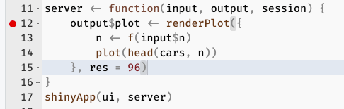{#fig-05-04fig-alt="alt-text" fig-align="center" width="70%"}If you’re using RStudio, the toolbar in @fig-05-05 will appear at thetop of the console when you’re in the debugger. The toolbar is an easyway to remember the debugging commands that are now available to you.They’re also available outside of RStudio; you’ll just need to rememberthe one letter command to activate them. The three most useful commandsare:- **Next (press n)**: executes the next step in the function. Note that if you have a variable named `n`, you’ll need to use `print(n)` to display its value.- **Continue (press c)**: leaves interactive debugging and continues regular execution of the function. This is useful if you’ve fixed the bad state and want to check that the function proceeds correctly.- **Stop (press Q)**: stops debugging, terminates the function, and returns to the global workspace. Use this once you’ve figured out where the problem is, and you’re ready to fix it and reload the code.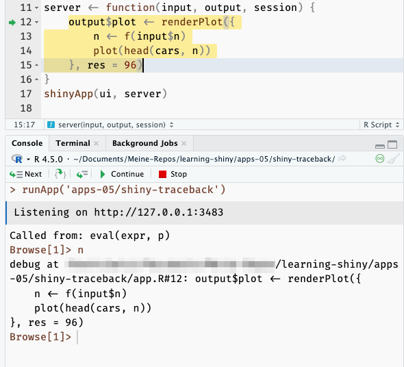{#fig-05-05fig-alt="alt-text" fig-align="center" width="70%"}As well as stepping through the code line-by-line using these tools,you’ll also write and run a bunch of interactive code to track downwhat’s going wrong. Debugging is the process of systematically comparingyour expectations to reality until you find the mismatch. If you’re newto debugging in R, you might want to read the [Debugging chapter of“Advanced R”](https://adv-r.hadley.nz/debugging.html) to learn somegeneral techniques.:::::: my-resource:::: my-resource-header::: {#lem-05-debugging}: Debugging:::::::::: my-resource-containerI have collected some resources for interactive debugging in R.- Jenny Bryan video keynote at the rstudio::conf(2020): “[Object of type ‘closure’ is not subsettable](https://posit.co/resources/videos/object-of-type-closure-is-not-subsettable/)”.[^05-workflow-1]- Jenny Bryan [Additional material and links from the above talk](https://github.com/jennybc/debugging#readme) to introduce R debugging.- Jonathan McPherson (posit): [Debugging with the RStudio IDE](https://support.posit.co/hc/en-us/articles/205612627-Debugging-with-the-RStudio-IDE)- [RStudio User Guide on Debugging](https://docs.posit.co/ide/user/ide/guide/code/debugging.html)- Hadley Wickham: General advise and problem-solving strategies in[Debugging](https://adv-r.hadley.nz/debugging.html) (Chapter 22 in the second edition of the [Advanced R book](https://adv-r.hadley.nz/index.html)).- The {**rlang**} package is a [collection of frameworks and APIs for programming with R](https://rlang.r-lib.org/). (I've already learned about this package, but it seems that it is — at least at the moment, June 2025 — a resource for more experienced programmers than me.):::::::::[^05-workflow-1]: This is for me an incomprehensibe error message that I have already experienced several times. It helps very much to replace 'closure' with 'function'.### Case studyI skip over the interesting and illuminating case study becausereproducing the reported strategies is not educationally valuable. Iwould need my own problem to debug.::: callout-importantIn the case study there are two important learnings for me:1. Assuming some line of code is the trouble maker try to reproduce the problem in the console outside the debugger!2. Inside the debugger try the interactive console to verify if you are in problematic line of code!:::By the way: I ran over a similar problem as reported in the case study.Instead of confusing "NA" for North America with `NA` I had the [ISO3166](https://www.iso.org/iso-3166-country-codes.html) two lettercountry code (alpha2) with "NA". (See filteredc [dataset to "Namibia" inopendatasoft](https://public.opendatasoft.com/explore/dataset/countries-codes/table/?flg=en-us&q=namibia))### Debugging reactivityThe hardest type of problem to debug is when your reactives fire in anunexpected order. At this point in the book, we have relatively fewtools to recommend to help you debug this issue. In the next section,you’ll learn how to create a minimal `r glossary("reprex")` which iscrucial for this type of problem, and later in the book, you’ll learnmore about the underlying theory, and about tools like the [reactivityvisualizer](https://github.com/rstudio/reactlog) {**reactlog**}[@reactlog]. But for now, we’ll focus on a classic technique that’suseful here: “print” debugging.The basic idea of print debugging is to call `print()` whenever you needto understand when a part of your code is evaluated, and to show thevalues of important variables. We call this “print” debugging (becausein most languages you’d use a print function), but In R it makes moresense to use `message()`:- `base::print()` is designed for displaying vectors of data so it puts quotes around strings and starts the first line with "\[1\]".- `base::message()` sends its result to “standard error”, rather than “standard output”. These are technical terms describing output streams, which you don’t normally notice because they’re both displayed in the same way when running interactively. But if your app is hosted elsewhere, then output sent to “standard error” will be recorded in the logs.I also recommend coupling `message()` with the `glue()` function fromthe {**glue**} package, which makes it easy to interleave text andvalues in a message.[^05-workflow-2][^05-workflow-2]: As I am already comfortable to use `glue()` I skip the demonstration how to use the {**glue**} package.A final useful tool is `utils::str()`, which prints the detailedstructure of any object. This is particularly useful if you need todouble check you have the type of object that you expect.Summarized there are three tools for print debugging at this state ofthe notes:- `base::message()`- `glue::glue()`- `utils::str()`Here’s a toy app that shows off some of the basic ideas. Note how I usemessage() inside a reactive(): I have to perform the computation, sendthe message, and then return the previously computed value.:::::::::::::::: my-code-collection::::: my-code-collection-header::: my-code-collection-icon:::::: {#exm-05-print-debugging}: Toy example with print debugging:::::::::::::::::::: my-code-collection-container::::::::::: panel-tabset###### Version 1 (Hadley):::::: my-r-code:::: my-r-code-header::: {#cnj-05-print-debugging-hadley}: Toy example from the book:::::::::: my-r-code-container```{shinylive-r}#| standalone: true#| components: [editor, viewer]library(shiny)library(glue)ui<- fluidPage(sliderInput("x","x", value = 1, min = 0, max = 10),sliderInput("y","y", value = 2, min = 0, max = 10),sliderInput("z","z", value = 3, min = 0, max = 10),textOutput("total"))server<- function(input, output, session){observeEvent(input$x, {message(glue("Updating y from {input$y} to {input$x * 2}"))updateSliderInput(session,"y", value = input$x* 2)})total<- reactive({total<- input$x + input$y + input$zmessage(glue("New total is {total}"))total})output$total<- renderText({total()})}shinyApp(ui, server)```***I can't demonstrate printing the output inside a reactive code snippet with {**shinylive**} here. Only the output in the not reactive `output$total` will appear. So I faked the output with copy and paste from the online book:```markdownUpdating y from 2 to 2New total is 6```And if I drag the x slider to 3 I see```markdownUpdating y from 2 to 6New total is 8New total is 12```Don’t worry if you find the results a little surprising. ::: {.callout-note}Yes, in fact, this *is* surprising for me, as I get the new total twice! I’ll will wait to learn more about what’s going on in @sec-chap08 with the help of the reactive graph diagrams mentioned in @sec-03-reactive-graph.In the meanwhile I have in the next tab changed text and place of the messages in this toy example.::::::::::::###### Version 2 (my own example):::::: my-r-code:::: my-r-code-header::: {#cnj-05-print-debugging-my-own}: Toy example with my own print debugging messages:::::::::: my-r-code-container```{r}#| label: print-debugging-my-own#| eval: falselibrary(shiny)library(glue)ui <-fluidPage(sliderInput("x", "x", value =1, min =0, max =10),sliderInput("y", "y", value =2, min =0, max =10),sliderInput("z", "z", value =3, min =0, max =10),textOutput("total"))server <-function(input, output, session) {observeEvent(input$x, {updateSliderInput(session, "y", value = input$x *2) }) total <-reactive({ total <- input$x + input$y + input$zmessage(glue("New total is x+y+z = {input$x} + {input$y} + {input$z} = {total}")) total }) output$total <-renderText({total() })}shinyApp(ui, server)```***The printing command in the `total` reactive is easier to understand for me. But I think the places for the `message()` command in the book example are on those other places to show an specific behavior of the reactivity behavior of this Shiny toy example.```markdown> shiny::runApp('apps-05/print-debugging')Loading required package: shinyListening on http://127.0.0.1:7653# After started the appNew total is x+y+z = 1 + 2 + 3 = 6# After dragging the x slider to 3New total is x+y+z = 3 + 2 + 3 = 8New total is x+y+z = 3 + 6 + 3 = 12```::::::::::::::::::::::::::::::::::::::::::::::::## Getting helpI will shorten this section as I have already some experiences with `r glossary("reprex", "reprexes")`. I will focus on those points that are not so obvious for me.### Reprex basics {#sec-05-reprex-basics}**{reprex} package**: In the book the usage of the [{reprex} package](https://reprex.tidyverse.org/) is not mentioned. It is a very useful tool and simplifies the technical process of catching the code. I am using the {**reprex**} package [@reprex] with [RStudio addins](https://rstudio.github.io/rstudioaddins/), because that makes it much comfortable to use.### Making a reprexThis section does not mention the technical process but focuses on conceptional issues.Typically, the most challenging part of making your app work on someone else’s computer is eliminating the use of data that’s only stored on your computer. There are four useful patterns:#### Built-in datsetOften the data you’re using is not directly related to the problem, and you can instead use a built-in dataset like mtcars or iris.#### R Code datasetOther times, you might be able to write a little R code that creates a dataset that illustrates the problem:```{r}#| label: create-mydata-with-r-codemydata <-data.frame(x =1:5, y =c("a", "b", "c", "d", "e"))mydata```#### `dput()` datasetIf both of those techniques fail, you can turn your data into code with base::dput(). For example, `dput(mydata)` generates the code that will recreate `mydata```:```{r}#| label: create-mydata-with-dputdput(mydata)```Once you have that code, you can put this in your reprex to generate `mydata`:```{r}#| label: put-mydata-in-reprex-codemydata <-structure(list(x =1:5, y =structure(1:5, .Label =c("a", "b","c", "d", "e"), class ="factor")), class ="data.frame", row.names =c(NA,-5L))mydata```Often, running `dput()` on your original data will generate a huge amount of code, so find a subset of your data that illustrates the problem. The smaller the dataset that you supply, the easier it will be for others to help you with your problem.#### Complete projectIf reading data from disk seems to be an irreducible part of the problem, a strategy of last resort is to provide a complete project containing both an app.R and the needed data files. The best way to provide this is as a **RStudio project hosted on GitHub**, but failing that, you can carefully make a **zip file that can be run locally**. Make sure that you use relative paths (i.e. `read.csv("my-data.csv")` not `read.csv("c:\\my-user-name\\files\\my-data.csv"))` so that your code still works when run on a different computer.You should also consider the reader and spend some time formatting your code so that it’s easy to read. If you adopt the tidyverse style guide, you can automatically reformat your code using the {**styler**} package; that quickly gets your code to a place that’s easier to read.### Making a minimal reprexCreating the smallest possible reprex is particularly important for Shiny apps, which are often complicated. But — as Jenny Bryan mentioned in her talk (see @sec-05-talk-jeyy-brian) — creating a minimal reprex is both a science and an art.::: {.callout-tip #tip-05-making-minimal-reprex}###### Debugging strategy but also a way to make a minimal reprex- If you don’t know what part of your code is triggering the problem, a good way to find it is to remove sections of code from your application, piece by piece, until the problem goes away. - Alternatively, sometimes it’s simpler to start with a fresh, empty, app and progressively build it up until you find the problem once more.:::::: {.my-checklist}::::{.my-checklist-header} ::::: {.my-checklist-icon}::::::::::: {#tdo-05-reprex}:::::: : Take a final pass through your Reprex:::::::: {.my-checklist-body} - Is every input and output in UI related to the problem?- Does your app have a complex layout that you can simplify to help focus on the problem at hand? Have you removed all UI customisation that makes your app look good, but isn’t related to the problem?- Are there any reactives in `server()` that you can now remove?- If you’ve tried multiple ways to solve the problem, have you removed all the vestiges of the attempts that didn’t work?- Is every package that you load needed to illustrate the problem? Can you eliminate packages by replacing functions with dummy code?:::::::### Case StudyAgain I will skip the case study, especially as I can't demonstrate it with a {**shinylive*} chunk. But I have provided the shiny apps in the "app05" folder.Another remark: I got slightly different error messages. For instance instead of "“Type mismatch for min, max, and value. Each must be Date, POSIXt, or number” in the first case study example I got "Error in min: invalid 'type' (list) of argument" with my experiment in the console.## SummaryThis chapter has given you some useful workflows for developing apps, debugging problems, and getting help. These workflows might seem a little abstract and easy to dismiss because they’re not concretely improving an individual app. But I think of workflow as one of my “secret” powers: one of the reasons that I’ve been able to accomplish so much is that I devote time to analysing and improving my workflow. I highly encourage you to do the same!The next chapter on layouts and themes is the first of a grab bag of useful techniques. There’s no need to read in sequence; feel free to skip ahead to a chapter that you need for a current app.::: {.callout-note #nte-next-chapter}I will follow the advice and continue with #sec-chap09 because I need the upload of a dataset for the work on my first real Shiny app.:::## Glossary Entries {#unnumbered}```{r}#| label: glossary-table#| echo: falseglossary_table()```------------------------------------------------------------------------## Session Info {.unnumbered}::: my-r-code::: my-r-code-headerSession Info:::::: my-r-code-container```{r}#| label: session-infosessioninfo::session_info()```::::::


