34 Day 33 (July 28)
34.1 Announcements
- Will update grades this afternoon
- TEVALS
- Final presentations
- If you don’t have a time or have not heard back from me, send me an email!
- Selected questions from journals
- “I just want to check if I’m getting this right: Model checking is when we evaluate how well the model fits the data we used to build it. We look at whether the model assumptions (like normality, independence, and homoscedasticity) are met, and we can also check things like accuracy or mean absolute error on the training data. Model validation, on the other hand, is about seeing how well the model works on new, unseen data. For that, we use methods like calibration, accuracy, AIC/BIC, R², and MAE on the test data.”
- “From my own understanding, model checking assesses if model assumptions are met as well as if the modelfits our data well, while model validation check how well the model perform on unseen data. Am I thinking right? When we calculate the MeanAbsolute Error to see prediction accuracy, this can be part of both model checking and validation right?”
34.2 Constant variance
If \(\mathbf{y}\sim\text{N}(\mathbf{X\boldsymbol{\beta}},\sigma^{2}\mathbf{I})\), then each \(\varepsilon_i\) follows a normal distribution with the same value of \(\sigma^2\).
- A linear model with constant variance is the simplest possible model we could assume. It is like the intercept only model in that regard.
- Example: Hubble data
##      2.5 %   97.5 %
## x 68.37937 84.78297
# Plot data and E(y) plot(hubble$x,hubble$y,xlab="Distance (Mpc)", ylab=expression("Velocity (km"*s^{-1}*")"),pch=20) abline(m1)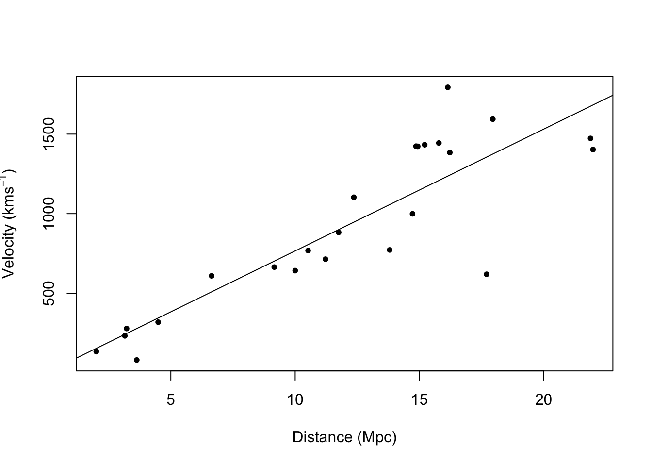
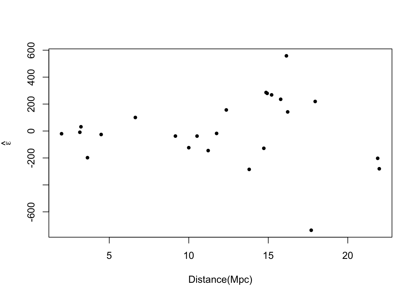
# Plot residuals vs. x
e.hat <- residuals(m1)
hist(e.hat,col="grey",breaks=15,main="",xlab=expression(hat(epsilon)))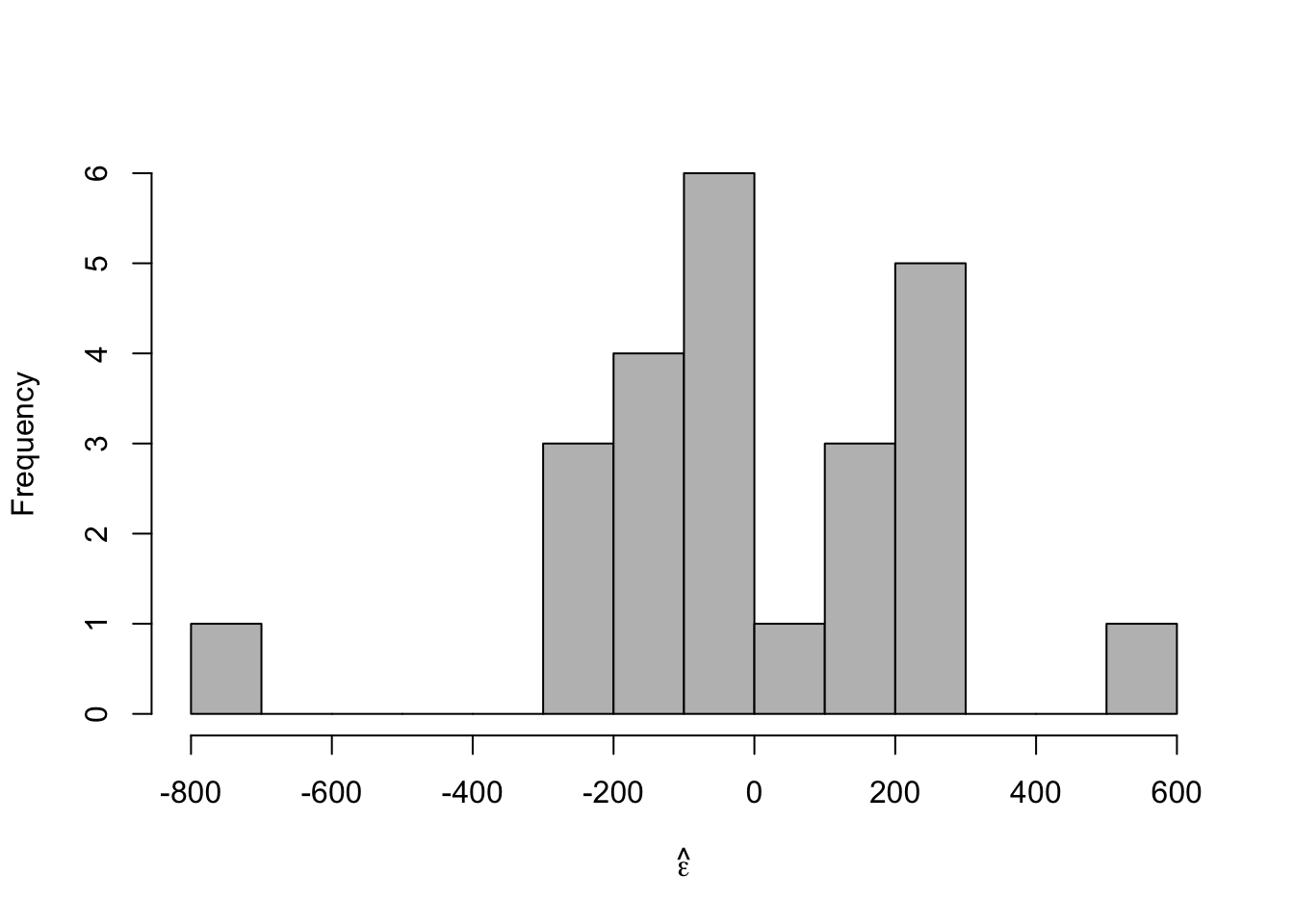
# Plot prediction intervals
y.pi <- predict(m1,newdata=data.frame(x = 0:25),interval = "predict")
plot(hubble$x,hubble$y,xlab="Distance (Mpc)",
ylab=expression("Velocity (km"*s^{-1}*")"),xlim=c(0,25),ylim=c(0,2500),pch=20)
points(0:25,y.pi[,2],typ="l",lwd=2,col="purple")
points(0:25,y.pi[,3],typ="l",lwd=2,col="purple")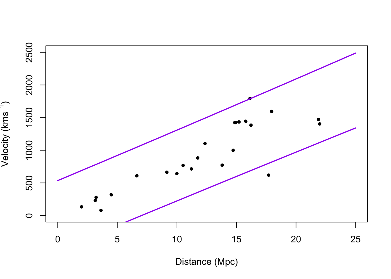
- A test for equal variance (see pg. 77 in Faraway (2014))
- What causes non-constant variance (also called heteroskedasticity).
What can be done?
- A transformation may work (see pg. 77 Faraway (2014))
- Build a more appropriate model for the variance. For example, \[\mathbf{y}\sim\text{N}(\mathbf{X\boldsymbol{\beta}},\mathbf{V})\] where the \(i^\text{th}\) and \(j^{th}\) entry of the matrix \(\mathbf{V}\) equals \[v_{ij}(\theta)=\begin{cases} \sigma^{2}e^{2\theta x_i} &\text{if}\ i=j\\ 0 &\text{if}\ i\neq j \end{cases}\]
## Generalized least squares fit by REML ## Model: y ~ x - 1 ## Data: hubble ## AIC BIC logLik ## 322.432 325.8385 -158.216 ## ## Variance function: ## Structure: Exponential of variance covariate ## Formula: ~x ## Parameter estimates: ## expon ## 0.1060336 ## ## Coefficients: ## Value Std.Error t-value p-value ## x 76.2548 3.854585 19.78288 0 ## ## Standardized residuals: ## Min Q1 Med Q3 Max ## -2.4272668 -0.4726915 -0.1548023 0.7929118 1.8437320 ## ## Residual standard error: 55.17695 ## Degrees of freedom: 24 total; 23 residual## 2.5 % 97.5 % ## x 68.69995 83.80965# Plot prediction intervals X <- model.matrix(y ~ x - 1, data = hubble) sigma2.hat <- summary(m1)$sigma^2 sigma2.hat * solve(t(X) %*% X)## x ## x 15.71959## x ## x 15.71959X <- model.matrix(y ~ x - 1, data = hubble) beta.hat <- coef(m2) sigma2.hat <- summary(m2)$sigma^2 theta.hat <- summary(m2)$modelStruct$varStruct V <- diag(c(sigma2.hat * exp(2 * X %*% theta.hat))) X.new <- model.matrix(~x - 1, data = data.frame(x = 1:25)) y.pi <- cbind(X.new %*% beta.hat - qt(0.975, 24 - 1) * sqrt(X.new^2 %*% solve(t(X) %*% solve(V) %*% X) + sigma2.hat * exp(2 * X.new %*% theta.hat)), X.new %*% beta.hat + qt(0.975, 24 - 1) * sqrt(X.new^2 %*% solve(t(X) %*% solve(V) %*% X) + sigma2.hat * exp(2 * X.new %*% theta.hat))) plot(hubble$x, hubble$y, xlab = "Distance (Mpc)", ylab = expression("Velocity (km" * s^{ -1 } * ")"), xlim = c(0, 25), ylim = c(0, 2500), pch = 20) points(1:25, y.pi[, 1], typ = "l", lwd = 2, col = "purple") points(1:25, y.pi[, 2], typ = "l", lwd = 2, col = "purple")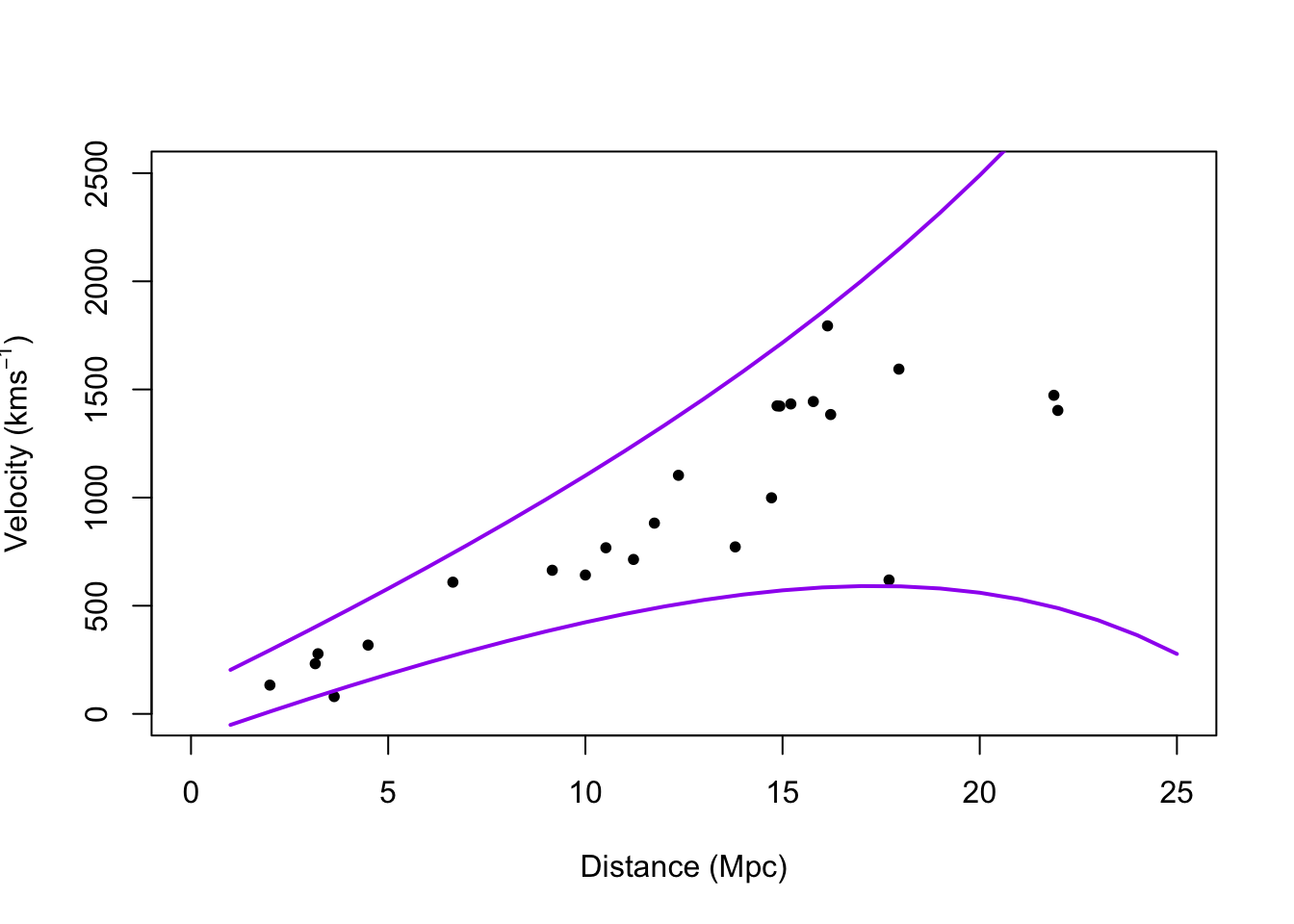
Example: Schizophrenia data
url <- "https://www.dropbox.com/scl/fi/y244p5qblopthh6nf5h8w/reaction_time.csv?rlkey=fvlqibqv990nzm957zy3qanxc&dl=1"
df1 <- read.csv(url)
head(df1)
## time schizophrenia ## 1 312 no ## 2 272 no ## 3 350 no ## 4 286 no ## 5 268 no ## 6 328 noboxplot(time ~ schizophrenia, data = df1, xlab = "Schizophrenic", ylab = "Reaction time (in milliseconds)")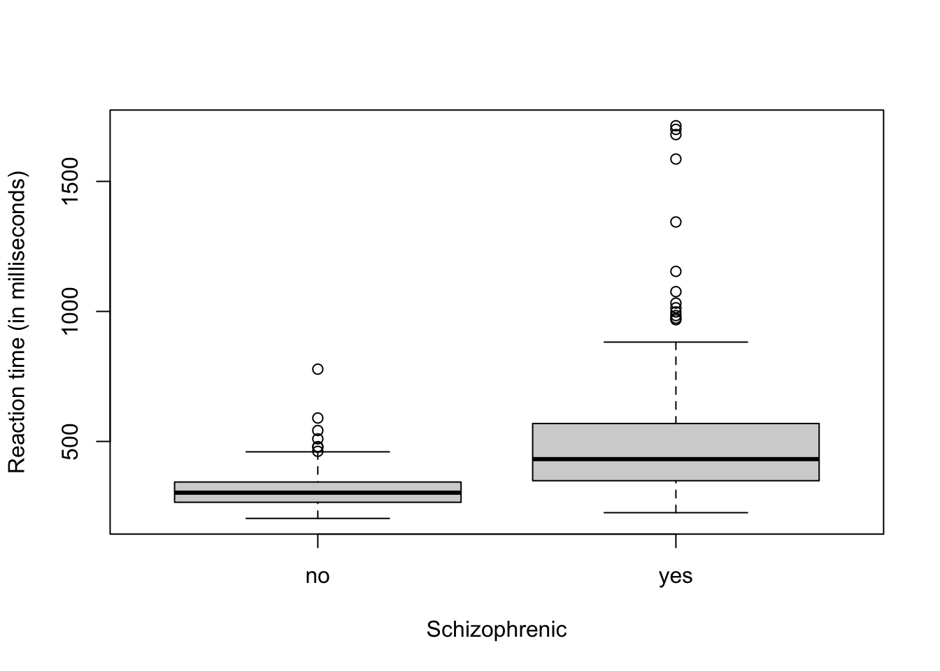
Example
- Linear model with constant variance
## ## Call: ## lm(formula = time ~ schizophrenia, data = df1) ## ## Residuals: ## Min 1Q Median 3Q Max ## -280.87 -70.17 -16.52 37.66 1207.13 ## ## Coefficients: ## Estimate Std. Error t value Pr(>|t|) ## (Intercept) 310.170 9.057 34.25 <2e-16 *** ## schizophreniayes 196.697 15.245 12.90 <2e-16 *** ## --- ## Signif. codes: 0 '***' 0.001 '**' 0.01 '*' 0.05 '.' 0.1 ' ' 1 ## ## Residual standard error: 164.5 on 508 degrees of freedom ## Multiple R-squared: 0.2468, Adjusted R-squared: 0.2453 ## F-statistic: 166.5 on 1 and 508 DF, p-value: < 2.2e-16- Plot residuals vs. predictor to check assumptions

- Plot residuals for each category
par(mfrow = c(2, 1))
hist(e.hat[which(x == 0)], col = "grey", xlab = expression(hat(epsilon)), main = expression(hat(epsilon) *
    " for x = 0"), xlim = c(range(e.hat)), breaks = seq(min(e.hat), max(e.hat), length.out = 40))
hist(e.hat[which(x == 1)], col = "grey", xlab = expression(hat(epsilon)), main = expression(hat(epsilon) *
    " for x = 1"), xlim = c(range(e.hat)), breaks = seq(min(e.hat), max(e.hat), length.out = 40))
- Looks like there are some outliers due to skewness in the distribution of \(\mathbf{y}\) and the variance is not constant. Let’s tackle the problem of non-constant variance first.
- Some possible solutions
- Build a more appropriate model for the variance. For example, \[\mathbf{y}\sim\text{N}(\mathbf{X\boldsymbol{\beta}},\mathbf{V})\] where the \(i^\text{th}\) and \(j^{th}\) entry of the matrix \(\mathbf{V}\) equals \[v_{ij}(\theta)=\begin{cases} \sigma^{2}e^{2\theta x_i} &\text{if}\ i=j\\ 0 &\text{if}\ i\neq j \end{cases}\]
- For additional options see
?varClassesafter loading the nlme package in R. - Fit model using
?glsfunction
library(nlme)
x <- ifelse(df1$schizophrenia == "no", 0, 1)
m2 <- gls(time ~ schizophrenia, weights = varExp(form = ~x), method = "REML", data = df1)
summary(m2)
## Generalized least squares fit by REML ## Model: time ~ schizophrenia ## Data: df1 ## AIC BIC logLik ## 6200.793 6217.715 -3096.396 ## ## Variance function: ## Structure: Exponential of variance covariate ## Formula: ~x ## Parameter estimates: ## expon ## 1.399026 ## ## Coefficients: ## Value Std.Error t-value p-value ## (Intercept) 310.1697 3.571554 86.84447 0 ## schizophreniayes 196.6970 19.914372 9.87714 0 ## ## Correlation: ## (Intr) ## schizophreniayes -0.179 ## ## Standardized residuals: ## Min Q1 Med Q3 Max ## -1.6363885 -0.6461803 -0.1875710 0.4166345 7.2106463 ## ## Residual standard error: 64.8805 ## Degrees of freedom: 510 total; 508 residual## lower est. upper ## expon 1.270298 1.399026 1.527755 ## attr(,"label") ## [1] "Variance function:"# See ?varExp theta.hat <- m2$model[1]$varStruct * 2 sigma2.hat <- summary(m2)$sigma^2 sigma2.hat * exp(theta.hat * 0)## Variance function structure of class varExp representing ## expon ## 4209.479## Variance function structure of class varExp representing ## expon ## 69088.72## [1] 4209.479## [1] 69088.72# p-value from glm should be the same as t-test with unequal variances t.test(time ~ schizophrenia, alternative = c("two.sided"), mu = 0, var.equal = FALSE, data = df1)## ## Welch Two Sample t-test ## ## data: time by schizophrenia ## t = -9.8771, df = 190.98, p-value < 2.2e-16 ## alternative hypothesis: true difference in means between group no and group yes is not equal to 0 ## 95 percent confidence interval: ## -235.9773 -157.4166 ## sample estimates: ## mean in group no mean in group yes ## 310.1697 506.8667# Conclusiongs from var.test should match up with m2 var.test(time ~ schizophrenia, alternative = c("two.sided"), data = df1)## ## F test to compare two variances ## ## data: time by schizophrenia ## F = 0.060929, num df = 329, denom df = 179, p-value < 2.2e-16 ## alternative hypothesis: true ratio of variances is not equal to 1 ## 95 percent confidence interval: ## 0.04683408 0.07847916 ## sample estimates: ## ratio of variances ## 0.0609286- Plot residuals vs. predictor to check assumption

- Plot residuals for each category
par(mfrow = c(2, 1))
hist(e.hat[which(x == 0)], col = "grey", xlab = expression(hat(epsilon)), main = expression(hat(epsilon) *
    " for x = 0"), xlim = c(range(e.hat)), breaks = seq(min(e.hat), max(e.hat), length.out = 40))
hist(e.hat[which(x == 1)], col = "grey", xlab = expression(hat(epsilon)), main = expression(hat(epsilon) *
    " for x = 1"), xlim = c(range(e.hat)), breaks = seq(min(e.hat), max(e.hat), length.out = 40))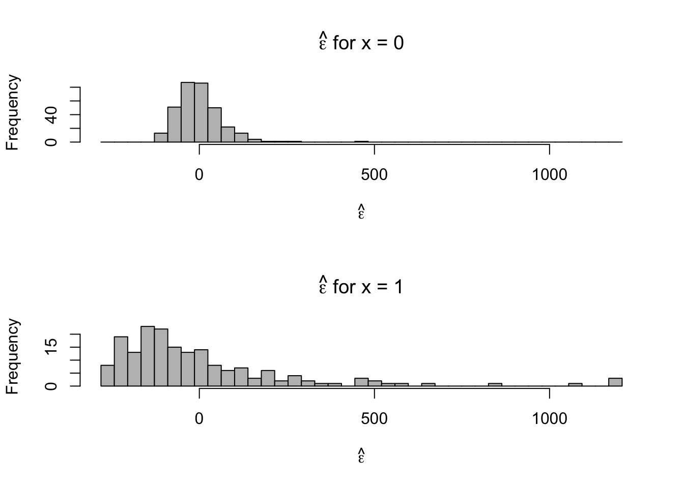
- Normal distribution is symmetric, the support of reaction times is always positive. We probably won’t be able to alleviate the issue of skewness using the normal distribution.
34.3 Collinearity
When two or more of the predictor variables (i.e., columns of \(\mathbf{X}\)) are correlated, the predictors are said to be collinear. Also called
- Collinearity
- Multicollinearity
- Correlation among predictors/covariates
- Partial parameter identifiability
Collinearity cause coefficient estimates (i.e., \(\hat{\boldsymbol{\beta}}\) to change when a collinear predictor is removed (or added) to the model.
- Extremely common problem with observational data and data collected from poorly designed experiments.
Example
- The data
library(httr)
library(readxl)

url <- "https://doi.org/10.1371/journal.pone.0148743.s005"
GET(url, write_disk(path <- tempfile(fileext = ".xls")))
df1 <- read_excel(path = path, sheet = "Data", col_names = TRUE, col_types = "numeric") notes <- read_excel(path = path, sheet = "Notes", col_names = FALSE)## # A tibble: 6 × 9 ## States Year CDEP WKIL WPOP BRPA NCAT SDEP NSHP ## <dbl> <dbl> <dbl> <dbl> <dbl> <dbl> <dbl> <dbl> <dbl> ## 1 1 1987 6 4 10 2 9736 10 1478 ## 2 1 1988 0 0 14 1 9324 0 1554 ## 3 1 1989 3 1 12 1 9190 0 1572 ## 4 1 1990 5 1 33 3 8345 0 1666 ## 5 1 1991 2 0 29 2 8733 2 1639 ## 6 1 1992 1 0 41 4 9428 0 1608## # A tibble: 9 × 2 ## ...1 ...2 ## <chr> <chr> ## 1 Year <NA> ## 2 State 1=Montana,2=Wyoming,3=Idaho ## 3 Cattle depredated CDEP ## 4 Sheep depredated SDEP ## 5 Wolf population WPOP ## 6 Wolves killed WKIL ## 7 Breeding pairs BRPA ## 8 Number of cattleA* NCAT ## 9 Number of SheepB* NSHPFit a linear model
## ## Call: ## lm(formula = CDEP ~ NCAT + WPOP, data = df1) ## ## Residuals: ## Min 1Q Median 3Q Max ## -40.289 -8.147 -3.475 2.678 92.257 ## ## Coefficients: ## Estimate Std. Error t value Pr(>|t|) ## (Intercept) -3.8455597 8.1697216 -0.471 0.64 ## NCAT 0.0009372 0.0010363 0.904 0.37 ## WPOP 0.1031119 0.0119644 8.618 7.51e-12 *** ## --- ## Signif. codes: 0 '***' 0.001 '**' 0.01 '*' 0.05 '.' 0.1 ' ' 1 ## ## Residual standard error: 20.23 on 56 degrees of freedom ## (3 observations deleted due to missingness) ## Multiple R-squared: 0.5855, Adjusted R-squared: 0.5707 ## F-statistic: 39.55 on 2 and 56 DF, p-value: 1.951e-11- Killing wolves should reduce the number of cattle depredated, right? Let’s add the number of wolves killed to our model.
## ## Call: ## lm(formula = CDEP ~ NCAT + WPOP + WKIL, data = df1) ## ## Residuals: ## Min 1Q Median 3Q Max ## -18.519 -8.549 -1.588 4.049 79.041 ## ## Coefficients: ## Estimate Std. Error t value Pr(>|t|) ## (Intercept) 13.901373 6.511267 2.135 0.0372 * ## NCAT -0.001385 0.000830 -1.669 0.1008 ## WPOP 0.011868 0.015724 0.755 0.4536 ## WKIL 0.683946 0.097769 6.996 3.84e-09 *** ## --- ## Signif. codes: 0 '***' 0.001 '**' 0.01 '*' 0.05 '.' 0.1 ' ' 1 ## ## Residual standard error: 14.85 on 55 degrees of freedom ## (3 observations deleted due to missingness) ## Multiple R-squared: 0.7807, Adjusted R-squared: 0.7687 ## F-statistic: 65.25 on 3 and 55 DF, p-value: < 2.2e-16- What happened?!
##             WKIL       WPOP        NCAT
## WKIL  1.00000000  0.7933354 -0.04460099
## WPOP  0.79333543  1.0000000 -0.34440797
## NCAT -0.04460099 -0.3444080  1.00000000
Some analytical results
- Assume the linear model \[\mathbf{y}=\beta_{1}\mathbf{x}+\beta_{2}\mathbf{z}+\boldsymbol{\varepsilon}\] where \(\boldsymbol{\varepsilon}\sim\text{N}(\mathbf{0},\sigma^{2}\mathbf{I})\)
- Assume that the predictors \(\mathbf{x}\) and \(\mathbf{z}\) are correlated (i.e., are not orthogonal \(\mathbf{x}^{\prime}\mathbf{z}\neq 0\) and \(\mathbf{z}^{\prime}\mathbf{x}\neq 0\)).
- Then \[\hat{\beta}_1 = (\mathbf{x}^{\prime}\mathbf{x}\times\mathbf{z}^{\prime}\mathbf{z} - \mathbf{x}^{\prime}\mathbf{z}\times\mathbf{z}^{\prime}\mathbf{x})^{-1}((\mathbf{z}^{\prime}\mathbf{z})\mathbf{x}^{\prime} - (\mathbf{x}^{\prime}\mathbf{z})\mathbf{z}^{\prime})\mathbf{y}\] and \[\hat{\beta}_2 = (\mathbf{z}^{\prime}\mathbf{z}\times\mathbf{x}^{\prime}\mathbf{x} - \mathbf{z}^{\prime}\mathbf{x}\times\mathbf{x}^{\prime}\mathbf{z})^{-1}((\mathbf{x}^{\prime}\mathbf{x})\mathbf{z}^{\prime} - (\mathbf{z}^{\prime}\mathbf{x})\mathbf{x}^{\prime})\mathbf{y}.\] The variance is \[\text{Var}(\hat{\beta}_{1})=\sigma^{2}\bigg{(}\frac{1}{1-R^{2}_{xz}}\bigg{)}\frac{1}{\sum_{i=1}^{n}(x_{i}-\bar{x})^{2}}\] \[\text{Var}(\hat{\beta}_{2})=\sigma^{2}\bigg{(}\frac{1}{1-R^{2}_{xz}}\bigg{)}\frac{1}{\sum_{i=1}^{n}(z_{i}-\bar{z})^{2}}\]where \(R^{2}_{xz}\) is the correlation between \(\mathbf{x}\) and \(\mathbf{z}\) (see pg. 107 in Faraway (2014)).
Take away message
- \(\hat{\beta}_i\) is the unbiased and minimum variance estimator assuming all predictors for \(\beta_i \neq 0\) are in the model.
- \(\hat{\beta}_i\) depends on the other predictors in the model.
- Correlation among predictors increases the variance of \(\hat{\beta}_i\).
- Known as the variance inflation factor
- Collinearity is ubiquitous in any model with correlated predictors
##     NCAT     WPOP     WKIL
## 1.350723 3.637257 3.212207
Literature cited
Faraway, J. J. 2014. Linear Models with r. CRC Press.