37 Day 36 (July 31)

37.1 Announcements

Today is the last day of class :(
Journal questions
- “Yesterday I believe I heard you say that the random effects regression penalizes the coefficients. I’m having difficulty in understanding why. Is it because the randomness of the error term negates the high coefficients of a model affected by collinearity? I’m not sure if I understand this right.”
- “I just want to check if I’m understanding this right: In GLMs, we don’t model the outcome directly. We model a transformation of its expected value using a link function. And to get the expected value of the outcome, we apply the inverse of the link function? How do we decide which link function to use? And how does that choice affect model fit?”
- “Is the statistical notation for generalized linear models read as: y follows a distribution of y given the expected value and dispersion, where a function of the expected value results in a linear order of parameters for predictors. Does this apply to each distribution? It seems the definition changed when we talked about binomial regression with the logit link, because y followed a distribution of outcomes and probability rather than expected value and dispersion.”

37.2 Generalized linear models

The generalized linear model framework \[\mathbf{y} \sim[\mathbf{\mathbf{y}|\boldsymbol{\mu},\psi]}\] \[g(\boldsymbol{\mu})=\mathbf{X}\boldsymbol{\beta}\]
- \([\mathbf{y}|\boldsymbol{\mu},\psi]\) is a distribution from the exponential family (e.g., normal, Poisson, binomial) with expected value \(\boldsymbol{\mu}\) and dispersion parameter \(\psi\).
  - Example \([\mathbf{y}|\boldsymbol{\mu},\psi]=\text{N}\left(\boldsymbol{\mu},\psi\mathbf{I}\right)\)
  - Example \([\mathbf{\mathbf{y}|\boldsymbol{\mu},\psi]}=\text{Poisson}\left(\boldsymbol{\mu}\right)\)
  - Example \([\mathbf{\mathbf{y}|\boldsymbol{\mu},\psi]}=\text{gamma}\left(\boldsymbol{\mu},\psi\right)\)

Estimation

Use numerical maximization to estimate
\(\hat{\boldsymbol{\beta}}=(\mathbf{X}^{\prime}\mathbf{X})^{-1}\mathbf{X}^{\prime}\mathbf{y}\) is NOT the MLE for the glm
Inference is based on asymptotic properties of MLE.
Example: Challenger data
- The statistical model: \[\mathbf{y}\sim\text{binomial}(6,\mathbf{p})\] \[\text{logit}(\mathbf{p})=\mathbf{X}\boldsymbol{\beta}.\]
- The PMF for the binomial distribution \[\binom{N}{y}p^{y}(1-p)^{N-y}\]
- Write out the likelihood function \[\mathcal{L}(\boldsymbol{\beta})=\prod_{i=1}^n\binom{6}{y_i}p_i^{y_i}(1-p_i)^{6-y_i}\]
Maximize the log-likelihood function

challenger <- read.csv("https://www.dropbox.com/s/ezxj8d48uh7lzhr/challenger.csv?dl=1")

plot(challenger$Temp,challenger$O.ring,xlab="Temperature",ylab="Number of incidents",xlim=c(10,80),ylim=c(0,6))

y <- challenger$O.ring
X <- model.matrix(~Temp,data= challenger)

nll <- function(beta){
  p <- 1/(1+exp(-X%*%beta)) # Inverse of logit link function
  -sum(dbinom(y,6,p,log=TRUE)) # Sum of the log likelihood for each observation 
  }
est <- optim(par=c(0,0),fn=nll,hessian=TRUE)

# MLE of beta
est$par

## [1]  6.751192 -0.139703

# Var(beta.hat)
diag(solve(est$hessian))

## [1] 8.830866682 0.002145791

# Std.Error
diag(solve(est$hessian))^0.5

## [1] 2.97167742 0.04632268

Using the glm() function

m1 <- glm(cbind(challenger$O.ring,6-challenger$O.ring) ~ Temp, family = binomial(link = "logit"),data=challenger)
summary(m1)

## 
## Call:
## glm(formula = cbind(challenger$O.ring, 6 - challenger$O.ring) ~ 
##     Temp, family = binomial(link = "logit"), data = challenger)
## 
## Coefficients:
##             Estimate Std. Error z value Pr(>|z|)   
## (Intercept)  6.75183    2.97989   2.266  0.02346 * 
## Temp        -0.13971    0.04647  -3.007  0.00264 **
## ---
## Signif. codes:  0 '***' 0.001 '**' 0.01 '*' 0.05 '.' 0.1 ' ' 1
## 
## (Dispersion parameter for binomial family taken to be 1)
## 
##     Null deviance: 28.761  on 22  degrees of freedom
## Residual deviance: 19.093  on 21  degrees of freedom
## AIC: 36.757
## 
## Number of Fisher Scoring iterations: 5

Prediction
- We can get prediction using \(\mathbf{X}\hat{\boldsymbol{\beta}}\) or the inverse of the logit link function \(\hat{\boldsymbol{\mu}}=\frac{1}{1+e^{-\mathbf{X}\hat{\boldsymbol{\beta}}}}\)
- Confidence intervals for \(\mathbf{X}\hat{\boldsymbol{\beta}}\) are straightforward
- Confidence intervals for \(\hat{\boldsymbol{\mu}}=\frac{1}{1+e^{-\mathbf{X}\hat{\boldsymbol{\beta}}}}\) are not straightforward because of the nonlinear transformation of \(\hat{\boldsymbol{\beta}}\)

beta.hat <- coef(m1)

new.temp <- seq(0,80,by=0.01)
X.new <- model.matrix(~new.temp)

mu.hat <- (1/(1+exp(-X.new%*%beta.hat)))

plot(challenger$Temp,challenger$O.ring,xlab="Temperature",ylab="Number of incidents",xlim=c(10,80),ylim=c(0,6))
points(new.temp,6*mu.hat,typ="l",col="red")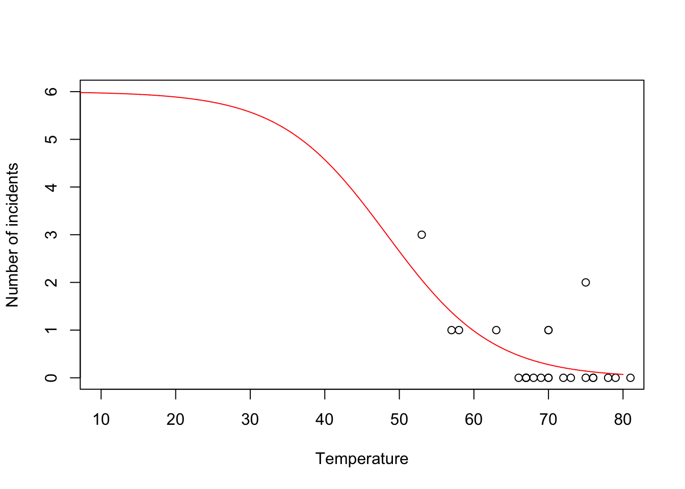

Predictive distribution

library(mosaic)

predict.bs <- function() {
    m1 <- glm(cbind(O.ring, 6 - O.ring) ~ Temp, family = binomial(link = "logit"),
        data = resample(challenger))
    p <- predict(m1, newdata = data.frame(Temp = 31), type = "response")
    y <- rbinom(1, 6, p)
    y
}

bootstrap <- do(1000) * predict.bs()

par(mar = c(5, 4, 7, 2))
hist(bootstrap[, 1], col = "grey", xlab = "Year", main = "Empirical distribution of O-ring failures at 31 degrees",
    freq = FALSE, right = FALSE, breaks = c(-0.5:6.5))

# 95% equal-tailed CI based on percentiles of the empirical distribution
quantile(bootstrap[, 1], prob = c(0.025, 0.975))

##  2.5% 97.5% 
##     0     6

# Proability of 6 O-rings failing
length(which(bootstrap[, 1] == 6))/dim(bootstrap)[1]

## [1] 0.521

Summary
- The generalized linear model useful when the distributional assumptions of linear model are untenable.
  - Small counts
  - Binary data
- Two cultures
  - All distributions are approximations of a unknown data generating process so why does it matter? Use the linear model because it is easier to understand.
  - Personal philosophy
    - Picking a distribution whose support matches that of the data gets closer to the etiology of the process that generated the data.
  - Easier for me to think scientifically about the process

37.3 Regression trees

Example: Change point analysis

Motivation: Annual mean temperature in Ann Arbor Michigan

library(faraway)
plot(aatemp$year, aatemp$temp, xlab = "Year", ylab = "Annual mean temperature", pch = 20,
    col = rgb(0.5, 0.5, 0.5, 0.7))

Basis function \[f_1(x)=\begin{cases} 1 & \text{if}\;x<c\\ 0 & \text{otherwise} \end{cases}\] and \[f_2(x)=\begin{cases} 1 & \text{if}\;x\geq c\\ 0 & \text{otherwise} \end{cases}\]
In R

# Change point basis function
f1 <- function(x, c) {
    ifelse(x < c, 1, 0)
}
f2 <- function(x, c) {
    ifelse(x >= c, 1, 0)
}

# Fit linear model
m1 <- lm(temp ~ -1 + f1(year, 1930) + f2(year, 1930), data = aatemp)
summary(m1)

## 
## Call:
## lm(formula = temp ~ -1 + f1(year, 1930) + f2(year, 1930), data = aatemp)
## 
## Residuals:
##     Min      1Q  Median      3Q     Max 
## -3.5467 -0.8962 -0.1157  1.1388  3.5843 
## 
## Coefficients:
##                Estimate Std. Error t value Pr(>|t|)    
## f1(year, 1930)  46.9567     0.1990   236.0   <2e-16 ***
## f2(year, 1930)  48.3057     0.1684   286.8   <2e-16 ***
## ---
## Signif. codes:  0 '***' 0.001 '**' 0.01 '*' 0.05 '.' 0.1 ' ' 1
## 
## Residual standard error: 1.378 on 113 degrees of freedom
## Multiple R-squared:  0.9992, Adjusted R-squared:  0.9992 
## F-statistic: 6.899e+04 on 2 and 113 DF,  p-value: < 2.2e-16

# Plot predictions
plot(aatemp$year, aatemp$temp, xlab = "Year", ylab = "Annual mean temperature", pch = 20,
    col = rgb(0.5, 0.5, 0.5, 0.7))
points(aatemp$year, predict(m1), type = "l")

Connection to regression trees
- For a single predictor, a regression tree can be though of as a linear model that uses the “change point” basis function, but tries to estimate the location (or time) and number of change points.
- Example in R

library(rpart)

# Fit regression tree model
m2 <- rpart(temp ~ year, data = aatemp)

# Plot predictions
E.y <- predict(m2, data.frame(year = seq(1850, 2023, by = 1)))
plot(aatemp$year, aatemp$temp, xlab = "Year", ylab = "Annual mean temperature", pch = 20,
    col = rgb(0.5, 0.5, 0.5, 0.7), xlim = c(1850, 2023))
points(1850:2023, E.y, type = "l")

37.4 Random forest

Breiman 2001 link

Example

n.boot <- 1000  # Number of bootstrap samples
x.new = seq(1850, 2023, by = 1)  # New values of x that I want predicitons at
E.y <- matrix(, length(x.new), n.boot)  # Matrix to save predictions
x <- aatemp$year
y <- aatemp$temp

for (i in 1:n.boot) {

    # Resample data
    df.temp <- data.frame(y = y, x = x)[sample(1:length(y), replace = TRUE, size = 51),
        ]

    # Fit tree
    m1 <- rpart(y ~ x, data = df.temp)

    # Get and save predictions
    E.y[, i] <- predict(m1, data.frame(x = x.new))
}

plot(aatemp$year, aatemp$temp, xlab = "Year", ylab = "Annual mean temperature", pch = 20,
    col = rgb(0.5, 0.5, 0.5, 0.7), xlim = c(1850, 2023))



# Aggregate predictions
E.E.y <- rowMeans(E.y)
points(1850:2023, E.E.y, type = "l")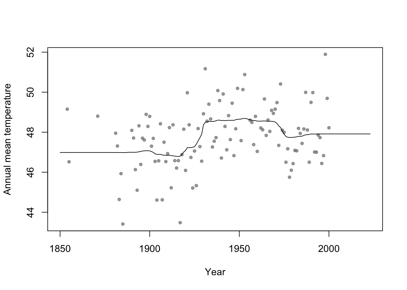

Summary
- Bootstrap aggregating (or bagging) can be used with any statistical model
- Usually increases predictive accuracy but reduces ability to understand (and write-out) the model(s) and make inference

37.5 Generalized additive model

Write out on white board
Difference between interpretable vs. non-interpretable model/machine learning approaches
My personal use of gams
- The functions lm() and glm() and packages lme4, nlme, etc
- Why I use the mgcv package
- Wood (2017)

Example

library(faraway)
library(mgcv)

m1 <- gam(temp ~ s(year, bs = "tp"), family = Gamma(link = "log"), data = aatemp)

# Plot predictions
E.y <- predict(m1, data.frame(year = seq(1850, 2023, by = 1)), type = "response")
ui <- E.y + 1.96 * predict(m1, data.frame(year = seq(1850, 2023, by = 1)), type = "response",
    se = TRUE)$se.fit
li <- E.y - 1.96 * predict(m1, data.frame(year = seq(1850, 2023, by = 1)), type = "response",
    se = TRUE)$se.fit
plot(aatemp$year, aatemp$temp, xlab = "Year", ylab = "Annual mean temperature", pch = 20,
    col = rgb(0.5, 0.5, 0.5, 0.7), xlim = c(1850, 2023))
points(1850:2023, E.y, type = "l", lwd = 3)
points(1850:2023, ui, type = "l", lwd = 2, lty = 2)
points(1850:2023, li, type = "l", lwd = 2, lty = 2)