35 Day 34 (July 29)
35.1 Announcements
- Grades should be up to date
- I will email you with your final grade before I submit any final grades
- Selected questions from journals
- “How advantageous, or how significant would that information be when at a conference? Would that depend on the type of data being presented? We don’t visualize and model variance much, but I can see why it is beneficial especially in animal trials.”
35.2 Collinearity
When two or more of the predictor variables (i.e., columns of \(\mathbf{X}\)) are correlated, the predictors are said to be collinear. Also called
- Collinearity
- Multicollinearity
- Correlation among predictors/covariates
- Partial parameter identifiability
Collinearity cause coefficient estimates (i.e., \(\hat{\boldsymbol{\beta}}\) to change when a collinear predictor is removed (or added) to the model.
- Extremely common problem with observational data and data collected from poorly designed experiments.
Example
- The data
library(httr)
library(readxl)

url <- "https://doi.org/10.1371/journal.pone.0148743.s005"
GET(url, write_disk(path <- tempfile(fileext = ".xls")))
df1 <- read_excel(path = path, sheet = "Data", col_names = TRUE, col_types = "numeric") notes <- read_excel(path = path, sheet = "Notes", col_names = FALSE)## # A tibble: 6 × 9 ## States Year CDEP WKIL WPOP BRPA NCAT SDEP NSHP ## <dbl> <dbl> <dbl> <dbl> <dbl> <dbl> <dbl> <dbl> <dbl> ## 1 1 1987 6 4 10 2 9736 10 1478 ## 2 1 1988 0 0 14 1 9324 0 1554 ## 3 1 1989 3 1 12 1 9190 0 1572 ## 4 1 1990 5 1 33 3 8345 0 1666 ## 5 1 1991 2 0 29 2 8733 2 1639 ## 6 1 1992 1 0 41 4 9428 0 1608## # A tibble: 9 × 2 ## ...1 ...2 ## <chr> <chr> ## 1 Year <NA> ## 2 State 1=Montana,2=Wyoming,3=Idaho ## 3 Cattle depredated CDEP ## 4 Sheep depredated SDEP ## 5 Wolf population WPOP ## 6 Wolves killed WKIL ## 7 Breeding pairs BRPA ## 8 Number of cattleA* NCAT ## 9 Number of SheepB* NSHPFit a linear model
## ## Call: ## lm(formula = CDEP ~ NCAT + WPOP, data = df1) ## ## Residuals: ## Min 1Q Median 3Q Max ## -40.289 -8.147 -3.475 2.678 92.257 ## ## Coefficients: ## Estimate Std. Error t value Pr(>|t|) ## (Intercept) -3.8455597 8.1697216 -0.471 0.64 ## NCAT 0.0009372 0.0010363 0.904 0.37 ## WPOP 0.1031119 0.0119644 8.618 7.51e-12 *** ## --- ## Signif. codes: 0 '***' 0.001 '**' 0.01 '*' 0.05 '.' 0.1 ' ' 1 ## ## Residual standard error: 20.23 on 56 degrees of freedom ## (3 observations deleted due to missingness) ## Multiple R-squared: 0.5855, Adjusted R-squared: 0.5707 ## F-statistic: 39.55 on 2 and 56 DF, p-value: 1.951e-11- Killing wolves should reduce the number of cattle depredated, right? Let’s add the number of wolves killed to our model.
## ## Call: ## lm(formula = CDEP ~ NCAT + WPOP + WKIL, data = df1) ## ## Residuals: ## Min 1Q Median 3Q Max ## -18.519 -8.549 -1.588 4.049 79.041 ## ## Coefficients: ## Estimate Std. Error t value Pr(>|t|) ## (Intercept) 13.901373 6.511267 2.135 0.0372 * ## NCAT -0.001385 0.000830 -1.669 0.1008 ## WPOP 0.011868 0.015724 0.755 0.4536 ## WKIL 0.683946 0.097769 6.996 3.84e-09 *** ## --- ## Signif. codes: 0 '***' 0.001 '**' 0.01 '*' 0.05 '.' 0.1 ' ' 1 ## ## Residual standard error: 14.85 on 55 degrees of freedom ## (3 observations deleted due to missingness) ## Multiple R-squared: 0.7807, Adjusted R-squared: 0.7687 ## F-statistic: 65.25 on 3 and 55 DF, p-value: < 2.2e-16- What happened?!
##             WKIL       WPOP        NCAT
## WKIL  1.00000000  0.7933354 -0.04460099
## WPOP  0.79333543  1.0000000 -0.34440797
## NCAT -0.04460099 -0.3444080  1.00000000
Some analytical results
- Assume the linear model \[\mathbf{y}=\beta_{1}\mathbf{x}+\beta_{2}\mathbf{z}+\boldsymbol{\varepsilon}\] where \(\boldsymbol{\varepsilon}\sim\text{N}(\mathbf{0},\sigma^{2}\mathbf{I})\)
- Assume that the predictors \(\mathbf{x}\) and \(\mathbf{z}\) are correlated (i.e., are not orthogonal \(\mathbf{x}^{\prime}\mathbf{z}\neq 0\) and \(\mathbf{z}^{\prime}\mathbf{x}\neq 0\)).
- Then \[\hat{\beta}_1 = (\mathbf{x}^{\prime}\mathbf{x}\times\mathbf{z}^{\prime}\mathbf{z} - \mathbf{x}^{\prime}\mathbf{z}\times\mathbf{z}^{\prime}\mathbf{x})^{-1}((\mathbf{z}^{\prime}\mathbf{z})\mathbf{x}^{\prime} - (\mathbf{x}^{\prime}\mathbf{z})\mathbf{z}^{\prime})\mathbf{y}\] and \[\hat{\beta}_2 = (\mathbf{z}^{\prime}\mathbf{z}\times\mathbf{x}^{\prime}\mathbf{x} - \mathbf{z}^{\prime}\mathbf{x}\times\mathbf{x}^{\prime}\mathbf{z})^{-1}((\mathbf{x}^{\prime}\mathbf{x})\mathbf{z}^{\prime} - (\mathbf{z}^{\prime}\mathbf{x})\mathbf{x}^{\prime})\mathbf{y}.\] The variance is \[\text{Var}(\hat{\beta}_{1})=\sigma^{2}\bigg{(}\frac{1}{1-R^{2}_{xz}}\bigg{)}\frac{1}{\sum_{i=1}^{n}(x_{i}-\bar{x})^{2}}\] \[\text{Var}(\hat{\beta}_{2})=\sigma^{2}\bigg{(}\frac{1}{1-R^{2}_{xz}}\bigg{)}\frac{1}{\sum_{i=1}^{n}(z_{i}-\bar{z})^{2}}\]where \(R^{2}_{xz}\) is the correlation between \(\mathbf{x}\) and \(\mathbf{z}\) (see pg. 107 in Faraway (2014)).
Take away message
- \(\hat{\beta}_i\) is the unbiased and minimum variance estimator assuming all predictors for \(\beta_i \neq 0\) are in the model.
- \(\hat{\beta}_i\) depends on the other predictors in the model.
- Correlation among predictors increases the variance of \(\hat{\beta}_i\).
- Known as the variance inflation factor
- Collinearity is ubiquitous in any model with correlated predictors
##     NCAT     WPOP     WKIL
## 1.350723 3.637257 3.212207
35.3 Random effects
Conditional, marginal, and joint distributions
- Conditional distribution: “\(\mathbf{y}\) given \(\boldsymbol{\beta}\)” \[\mathbf{y}|\boldsymbol{\beta}\sim\text{N}(\mathbf{X}\boldsymbol{\beta},\sigma_{\varepsilon}^{2}\mathbf{I})\] This is also sometimes called the data model.
- Marginal distribution of \(\boldsymbol{\beta}\) \[\beta\sim\text{N}(\mathbf{0},\sigma_{\beta}^{2}\mathbf{I})\] This is also called the parameter model.
- Joint distribution \([\mathbf{y}|\boldsymbol{\beta}][\boldsymbol{\beta}]\)
Estimation for the linear model with random effects
- By maximizing the joint likelihood
- Write out the likelihood function \[\mathcal{L}(\boldsymbol{\beta},\sigma_{\varepsilon},\sigma_{\beta}^{2})=\frac{1}{(2\pi)^{-\frac{n}{2}}}|\sigma^{2}_{\varepsilon}\mathbf{I}|^{-\frac{1}{2}}\text{exp}\bigg{(}-\frac{1}{2}(\mathbf{y} - \mathbf{X}\boldsymbol{\beta})^{\prime}(\sigma^{2}_{\varepsilon}\mathbf{I})^{-1}(\mathbf{y} - \mathbf{X}\boldsymbol{\beta})\bigg{)}\times\\\frac{1}{(2\pi)^{-\frac{p}{2}}}|\sigma^{2}_{\beta}\mathbf{I}|^{-\frac{1}{2}}\text{exp}\bigg{(}-\frac{1}{2}\boldsymbol{\beta}^{\prime}(\sigma^{2}_{\beta}\mathbf{I})^{-1}\boldsymbol{\beta}\bigg{)}\]
- Maximizing the log-likelihood function w.r.t. gives \(\boldsymbol{\beta}\) gives \[\hat{\boldsymbol{\beta}}=\big{(}\mathbf{X}^{'}\mathbf{X}+\frac{\sigma^{2}_{\varepsilon}}{\sigma^{2}_{\beta}}\mathbf{I}\big{)}^{-1}\mathbf{X}^{'}\mathbf{y}\]
- By maximizing the joint likelihood
Example eye temperature data set for Eurasian blue tit
df.et <- read.table("https://www.dropbox.com/s/bo11n66cezdnbia/eyetemp.txt?dl=1")
names(df.et) <- c("id", "sex", "date", "time", "event", "airtemp", "relhum", "sun",
    "bodycond", "eyetemp")
df.et$id <- as.factor(df.et$id)
df.et$id.num <- as.numeric(df.et$id)

ind.means <- aggregate(eyetemp ~ id.num, df.et, FUN = base::mean)
plot(df.et$id.num, df.et$eyetemp, xlab = "Individual", ylab = "Eye temperature")
points(ind.means, pch = "x", col = "gold", cex = 1.5)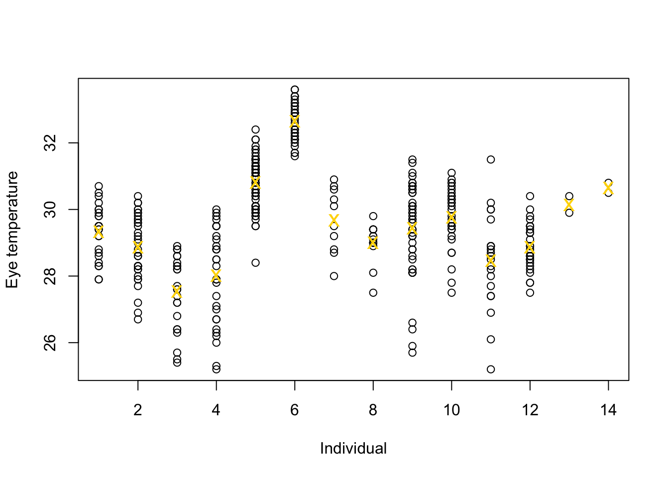
# Standard 'fixed effects' linear regression model
m1 <- lm(eyetemp ~ as.factor(id.num) - 1, data = df.et)
summary(m1)
## ## Call: ## lm(formula = eyetemp ~ as.factor(id.num) - 1, data = df.et) ## ## Residuals: ## Min 1Q Median 3Q Max ## -3.7378 -0.5750 0.1507 0.6622 3.0286 ## ## Coefficients: ## Estimate Std. Error t value Pr(>|t|) ## as.factor(id.num)1 29.3423 0.1972 148.77 <2e-16 *** ## as.factor(id.num)2 28.8735 0.1725 167.41 <2e-16 *** ## as.factor(id.num)3 27.5458 0.2053 134.19 <2e-16 *** ## as.factor(id.num)4 28.0156 0.1778 157.59 <2e-16 *** ## as.factor(id.num)5 30.8188 0.1211 254.56 <2e-16 *** ## as.factor(id.num)6 32.6486 0.1700 192.06 <2e-16 *** ## as.factor(id.num)7 29.6800 0.3180 93.33 <2e-16 *** ## as.factor(id.num)8 29.0000 0.2789 103.97 <2e-16 *** ## as.factor(id.num)9 29.4378 0.1499 196.36 <2e-16 *** ## as.factor(id.num)10 29.7667 0.1836 162.12 <2e-16 *** ## as.factor(id.num)11 28.4714 0.2195 129.74 <2e-16 *** ## as.factor(id.num)12 28.8793 0.1867 154.64 <2e-16 *** ## as.factor(id.num)13 30.1500 0.7111 42.40 <2e-16 *** ## as.factor(id.num)14 30.6500 0.7111 43.10 <2e-16 *** ## --- ## Signif. codes: 0 '***' 0.001 '**' 0.01 '*' 0.05 '.' 0.1 ' ' 1 ## ## Residual standard error: 1.006 on 358 degrees of freedom ## Multiple R-squared: 0.9989, Adjusted R-squared: 0.9989 ## F-statistic: 2.31e+04 on 14 and 358 DF, p-value: < 2.2e-16plot(df.et$id.num, df.et$eyetemp, xlab = "Individual", ylab = "Expected eye temperature", col = "white") points(1:14, coef(m1), pch = 20, col = "black", cex = 1) segments(1:14, confint(m1)[, 1], 1:14, confint(m1)[, 2], lwd = 2, lty = 1)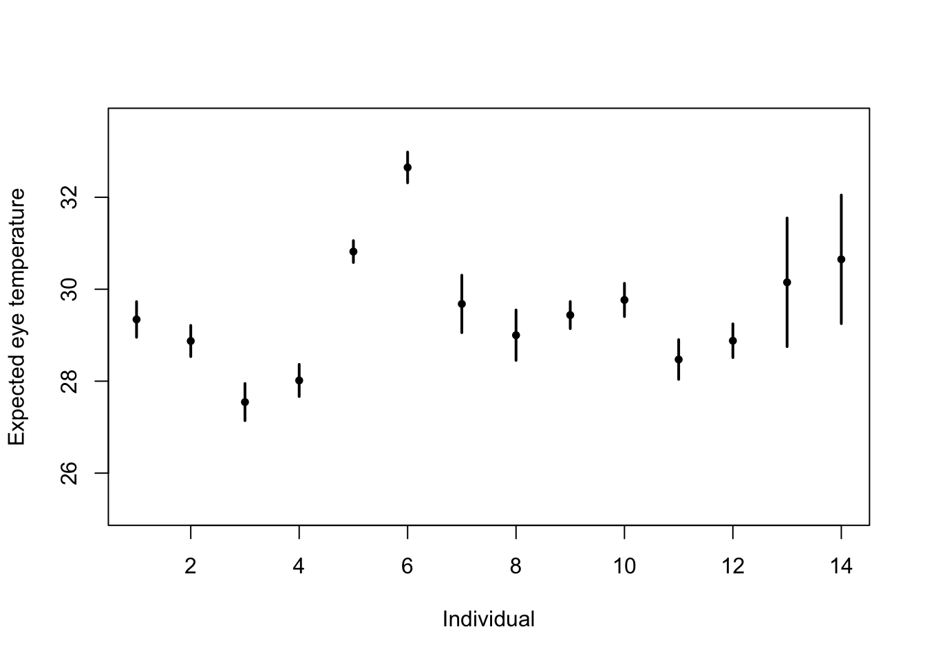
# Random effects regression model (using nlme package; difficult to get
# confidence interval)
library(nlme)
m2 <- lme(fixed = eyetemp ~ 1, random = list(id = pdIdent(~id - 1)), data = df.et,
    method = "ML")  #summary(m2)
# predict(m2,level=1,newdata=data.frame(id=unique(df.et$id)))

# Random effects regression model (mgcv package)
library(mgcv)
m2 <- gam(eyetemp ~ 1 + s(id, bs = "re"), data = df.et, method = "ML")

plot(df.et$id.num, df.et$eyetemp, xlab = "Individual", ylab = "Expected eye temperature",
    col = "white")
points(1:14 - 0.15, coef(m1), pch = 20, col = "black", cex = 1)
segments(1:14 - 0.15, confint(m1)[, 1], 1:14 - 0.15, confint(m1)[, 2], lwd = 2, lty = 1)
pred <- predict(m2, newdata = data.frame(id = unique(df.et$id)), se.fit = TRUE)
pred$lci <- pred$fit - 1.96 * pred$se.fit
pred$uci <- pred$fit + 1.96 * pred$se.fit
points(1:14 + 0.15, pred$fit, pch = 20, col = "green", cex = 1)
segments(1:14 + 0.15, pred$lci, 1:14 + 0.15, pred$uci, lwd = 2, lty = 1, col = "green")
abline(a = coef(m2)[1], b = 0, col = "grey")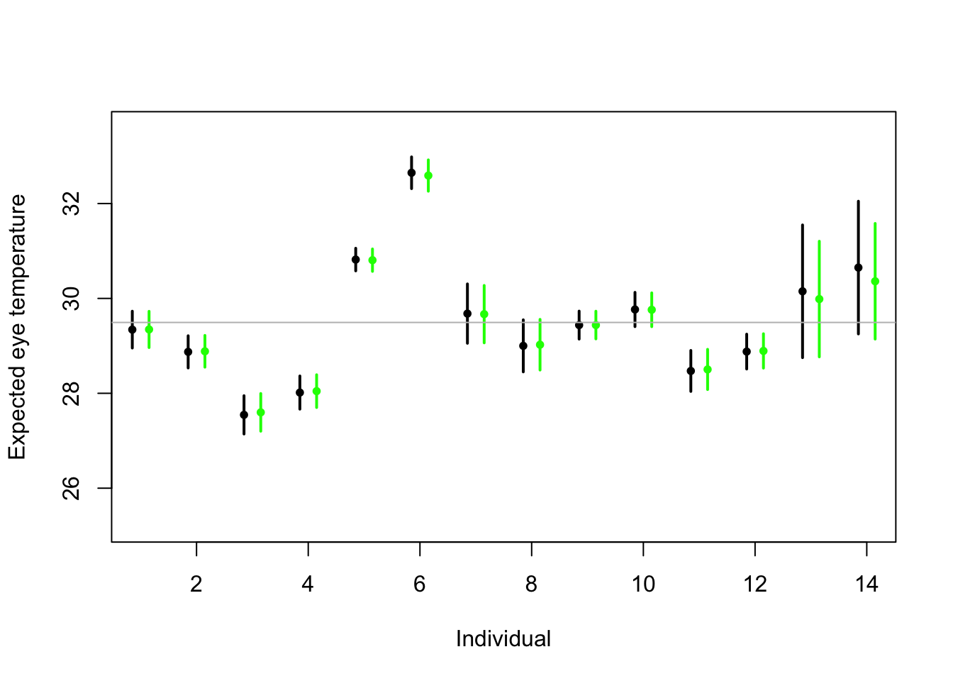
Summary
- Take home message
- Treating \(\boldsymbol{\beta}\) as a random effect “shrinks” the estimates of \(\boldsymbol{\beta}\) closer to zero.
- Requires an extra assumption \(\boldsymbol{\beta}\sim\text{N}(\mathbf{0},\sigma_{\beta}^{2}\mathbf{I})\)
- Penalty
- Random effect
- This called a prior distribution in Bayesian statistics
- Take home message
35.4 Generalized linear models
The generalized linear model framework \[\mathbf{y} \sim[\mathbf{\mathbf{y}|\boldsymbol{\mu},\psi]}\] \[g(\boldsymbol{\mu})=\mathbf{X}\boldsymbol{\beta}\]
- \([\mathbf{y}|\boldsymbol{\mu},\psi]\) is a distribution from the exponential family (e.g., normal, Poisson, binomial) with expected value \(\boldsymbol{\mu}\) and dispersion parameter \(\psi\).
- Example \([\mathbf{y}|\boldsymbol{\mu},\psi]=\text{N}\left(\boldsymbol{\mu},\psi\mathbf{I}\right)\)
- Example \([\mathbf{\mathbf{y}|\boldsymbol{\mu},\psi]}=\text{Poisson}\left(\boldsymbol{\mu}\right)\)
- Example \([\mathbf{\mathbf{y}|\boldsymbol{\mu},\psi]}=\text{gamma}\left(\boldsymbol{\mu},\psi\right)\)
- \([\mathbf{y}|\boldsymbol{\mu},\psi]\) is a distribution from the exponential family (e.g., normal, Poisson, binomial) with expected value \(\boldsymbol{\mu}\) and dispersion parameter \(\psi\).
Estimation
- Use numerical maximization to estimate
- \(\hat{\boldsymbol{\beta}}=(\mathbf{X}^{\prime}\mathbf{X})^{-1}\mathbf{X}^{\prime}\mathbf{y}\) is NOT the MLE for the glm
- Inference is based on asymptotic properties of MLE.
- Example: Challenger data
- The statistical model: \[\mathbf{y}\sim\text{binomial}(6,\mathbf{p})\] \[\text{logit}(\mathbf{p})=\mathbf{X}\boldsymbol{\beta}.\]
- The PMF for the binomial distribution \[\binom{N}{y}p^{y}(1-p)^{N-y}\]
- Write out the likelihood function \[\mathcal{L}(\boldsymbol{\beta})=\prod_{i=1}^n\binom{6}{y_i}p_i^{y_i}(1-p_i)^{6-y_i}\]
- Maximize the log-likelihood function
challenger <- read.csv("https://www.dropbox.com/s/ezxj8d48uh7lzhr/challenger.csv?dl=1")

plot(challenger$Temp,challenger$O.ring,xlab="Temperature",ylab="Number of incidents",xlim=c(10,80),ylim=c(0,6))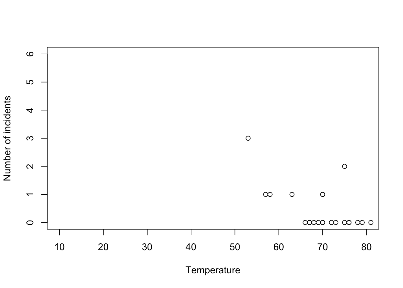
y <- challenger$O.ring
X <- model.matrix(~Temp,data= challenger)

nll <- function(beta){
  p <- 1/(1+exp(-X%*%beta)) # Inverse of logit link function
  -sum(dbinom(y,6,p,log=TRUE)) # Sum of the log likelihood for each observation
  }
est <- optim(par=c(0,0),fn=nll,hessian=TRUE)

# MLE of beta
est$par
## [1] 6.751192 -0.139703## [1] 8.830866682 0.002145791## [1] 2.97167742 0.04632268- Using the
glm()function
m1 <- glm(cbind(challenger$O.ring,6-challenger$O.ring) ~ Temp, family = binomial(link = "logit"),data=challenger)
summary(m1)
## ## Call: ## glm(formula = cbind(challenger$O.ring, 6 - challenger$O.ring) ~ ## Temp, family = binomial(link = "logit"), data = challenger) ## ## Coefficients: ## Estimate Std. Error z value Pr(>|z|) ## (Intercept) 6.75183 2.97989 2.266 0.02346 * ## Temp -0.13971 0.04647 -3.007 0.00264 ** ## --- ## Signif. codes: 0 '***' 0.001 '**' 0.01 '*' 0.05 '.' 0.1 ' ' 1 ## ## (Dispersion parameter for binomial family taken to be 1) ## ## Null deviance: 28.761 on 22 degrees of freedom ## Residual deviance: 19.093 on 21 degrees of freedom ## AIC: 36.757 ## ## Number of Fisher Scoring iterations: 5- Prediction
- We can get prediction using \(\mathbf{X}\hat{\boldsymbol{\beta}}\) or the inverse of the logit link function \(\hat{\boldsymbol{\mu}}=\frac{1}{1+e^{-\mathbf{X}\hat{\boldsymbol{\beta}}}}\)
- Confidence intervals for \(\mathbf{X}\hat{\boldsymbol{\beta}}\) are straightforward
- Confidence intervals for \(\hat{\boldsymbol{\mu}}=\frac{1}{1+e^{-\mathbf{X}\hat{\boldsymbol{\beta}}}}\) are not straightforward because of the nonlinear transformation of \(\hat{\boldsymbol{\beta}}\)
beta.hat <- coef(m1)

new.temp <- seq(0,80,by=0.01)
X.new <- model.matrix(~new.temp)

mu.hat <- (1/(1+exp(-X.new%*%beta.hat)))

plot(challenger$Temp,challenger$O.ring,xlab="Temperature",ylab="Number of incidents",xlim=c(10,80),ylim=c(0,6))
points(new.temp,6*mu.hat,typ="l",col="red")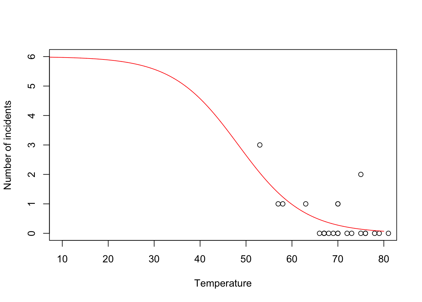
- Predictive distribution
library(mosaic)

predict.bs <- function() {
    m1 <- glm(cbind(O.ring, 6 - O.ring) ~ Temp, family = binomial(link = "logit"),
        data = resample(challenger))
    p <- predict(m1, newdata = data.frame(Temp = 31), type = "response")
    y <- rbinom(1, 6, p)
    y
}

bootstrap <- do(1000) * predict.bs()

par(mar = c(5, 4, 7, 2))
hist(bootstrap[, 1], col = "grey", xlab = "Year", main = "Empirical distribution of O-ring failures at 31 degrees",
    freq = FALSE, right = FALSE, breaks = c(-0.5:6.5))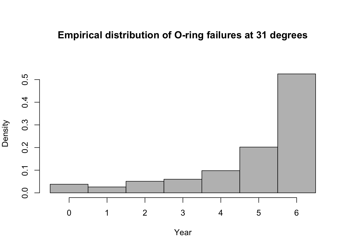
# 95% equal-tailed CI based on percentiles of the empirical distribution
quantile(bootstrap[, 1], prob = c(0.025, 0.975))
## 2.5% 97.5% ## 0 6## [1] 0.525Summary
- The generalized linear model useful when the distributional assumptions of linear model are untenable.
- Small counts
- Binary data
- Two cultures
- All distributions are approximations of a unknown data generating process so why does it matter? Use the linear model because it is easier to understand.
- Personal philosophy
- Picking a distribution whose support matches that of the data gets closer to the etiology of the process that generated the data.
- Easier for me to think scientifically about the process
- The generalized linear model useful when the distributional assumptions of linear model are untenable.
Literature cited
Faraway, J. J. 2014. Linear Models with r. CRC Press.