36 Day 35 (July 30)
36.1 Announcements
Presentations are going well!
Selected questions from journals
- General question about col linearity….every method is sensitive to collinearity
- “I understand that adding more assumptions should give us something back to make it worth it. And that’s not always the case with random effects. But how do we explain this to professors who are used to using them? The main thing we often hear is that if we consider something like location and block(location) as a random effect then we canmake broader inferences, for example, to all of Kansas. That’s the main reason I’veheard for why we should consider random effects.”
36.2 Random effects
Conditional, marginal, and joint distributions
- Conditional distribution: “\(\mathbf{y}\) given \(\boldsymbol{\beta}\)” \[\mathbf{y}|\boldsymbol{\beta}\sim\text{N}(\mathbf{X}\boldsymbol{\beta},\sigma_{\varepsilon}^{2}\mathbf{I})\] This is also sometimes called the data model.
- Marginal distribution of \(\boldsymbol{\beta}\) \[\beta\sim\text{N}(\mathbf{0},\sigma_{\beta}^{2}\mathbf{I})\] This is also called the parameter model.
- Joint distribution \([\mathbf{y}|\boldsymbol{\beta}][\boldsymbol{\beta}]\)
Estimation for the linear model with random effects
- By maximizing the joint likelihood
- Write out the likelihood function \[\mathcal{L}(\boldsymbol{\beta},\sigma_{\varepsilon},\sigma_{\beta}^{2})=\frac{1}{(2\pi)^{-\frac{n}{2}}}|\sigma^{2}_{\varepsilon}\mathbf{I}|^{-\frac{1}{2}}\text{exp}\bigg{(}-\frac{1}{2}(\mathbf{y} - \mathbf{X}\boldsymbol{\beta})^{\prime}(\sigma^{2}_{\varepsilon}\mathbf{I})^{-1}(\mathbf{y} - \mathbf{X}\boldsymbol{\beta})\bigg{)}\times\\\frac{1}{(2\pi)^{-\frac{p}{2}}}|\sigma^{2}_{\beta}\mathbf{I}|^{-\frac{1}{2}}\text{exp}\bigg{(}-\frac{1}{2}\boldsymbol{\beta}^{\prime}(\sigma^{2}_{\beta}\mathbf{I})^{-1}\boldsymbol{\beta}\bigg{)}\]
- Maximizing the log-likelihood function w.r.t. gives \(\boldsymbol{\beta}\) gives \[\hat{\boldsymbol{\beta}}=\big{(}\mathbf{X}^{'}\mathbf{X}+\frac{\sigma^{2}_{\varepsilon}}{\sigma^{2}_{\beta}}\mathbf{I}\big{)}^{-1}\mathbf{X}^{'}\mathbf{y}\]
- By maximizing the joint likelihood
Example eye temperature data set for Eurasian blue tit
df.et <- read.table("https://www.dropbox.com/s/bo11n66cezdnbia/eyetemp.txt?dl=1")
names(df.et) <- c("id", "sex", "date", "time", "event", "airtemp", "relhum", "sun",
    "bodycond", "eyetemp")
df.et$id <- as.factor(df.et$id)
df.et$id.num <- as.numeric(df.et$id)

ind.means <- aggregate(eyetemp ~ id.num, df.et, FUN = base::mean)
plot(df.et$id.num, df.et$eyetemp, xlab = "Individual", ylab = "Eye temperature")
points(ind.means, pch = "x", col = "gold", cex = 1.5)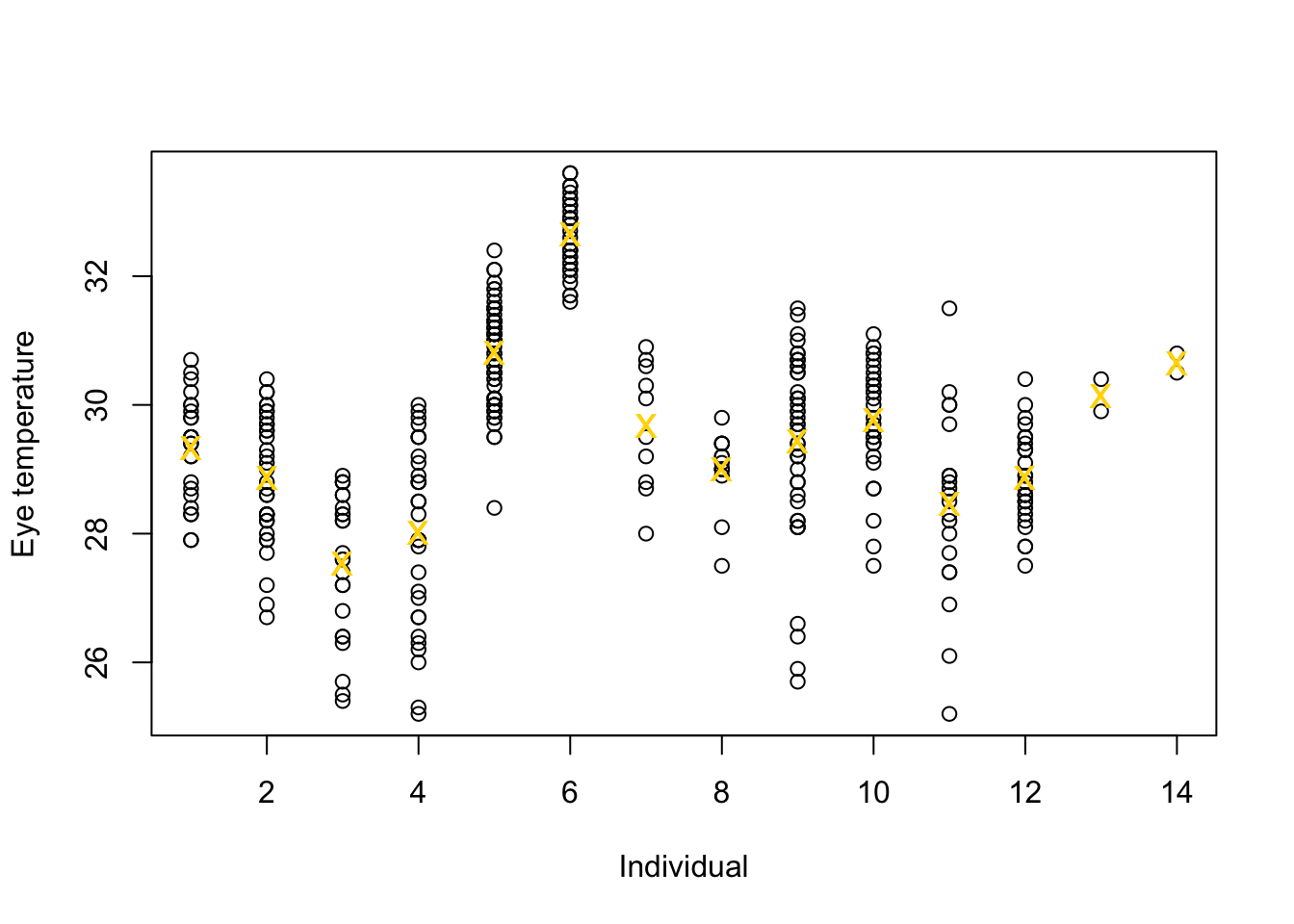
# Standard 'fixed effects' linear regression model
m1 <- lm(eyetemp ~ as.factor(id.num) - 1, data = df.et)
summary(m1)
## ## Call: ## lm(formula = eyetemp ~ as.factor(id.num) - 1, data = df.et) ## ## Residuals: ## Min 1Q Median 3Q Max ## -3.7378 -0.5750 0.1507 0.6622 3.0286 ## ## Coefficients: ## Estimate Std. Error t value Pr(>|t|) ## as.factor(id.num)1 29.3423 0.1972 148.77 <2e-16 *** ## as.factor(id.num)2 28.8735 0.1725 167.41 <2e-16 *** ## as.factor(id.num)3 27.5458 0.2053 134.19 <2e-16 *** ## as.factor(id.num)4 28.0156 0.1778 157.59 <2e-16 *** ## as.factor(id.num)5 30.8188 0.1211 254.56 <2e-16 *** ## as.factor(id.num)6 32.6486 0.1700 192.06 <2e-16 *** ## as.factor(id.num)7 29.6800 0.3180 93.33 <2e-16 *** ## as.factor(id.num)8 29.0000 0.2789 103.97 <2e-16 *** ## as.factor(id.num)9 29.4378 0.1499 196.36 <2e-16 *** ## as.factor(id.num)10 29.7667 0.1836 162.12 <2e-16 *** ## as.factor(id.num)11 28.4714 0.2195 129.74 <2e-16 *** ## as.factor(id.num)12 28.8793 0.1867 154.64 <2e-16 *** ## as.factor(id.num)13 30.1500 0.7111 42.40 <2e-16 *** ## as.factor(id.num)14 30.6500 0.7111 43.10 <2e-16 *** ## --- ## Signif. codes: 0 '***' 0.001 '**' 0.01 '*' 0.05 '.' 0.1 ' ' 1 ## ## Residual standard error: 1.006 on 358 degrees of freedom ## Multiple R-squared: 0.9989, Adjusted R-squared: 0.9989 ## F-statistic: 2.31e+04 on 14 and 358 DF, p-value: < 2.2e-16plot(df.et$id.num, df.et$eyetemp, xlab = "Individual", ylab = "Expected eye temperature", col = "white") points(1:14, coef(m1), pch = 20, col = "black", cex = 1) segments(1:14, confint(m1)[, 1], 1:14, confint(m1)[, 2], lwd = 2, lty = 1)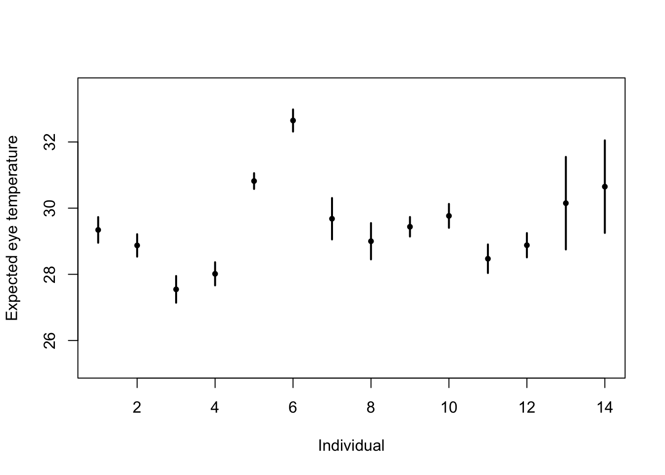
# Random effects regression model (using nlme package; difficult to get
# confidence interval)
library(nlme)
m2 <- lme(fixed = eyetemp ~ 1, random = list(id = pdIdent(~id - 1)), data = df.et,
    method = "ML")  #summary(m2)
# predict(m2,level=1,newdata=data.frame(id=unique(df.et$id)))

# Random effects regression model (mgcv package)
library(mgcv)
m2 <- gam(eyetemp ~ 1 + s(id, bs = "re"), data = df.et, method = "ML")

plot(df.et$id.num, df.et$eyetemp, xlab = "Individual", ylab = "Expected eye temperature",
    col = "white")
points(1:14 - 0.15, coef(m1), pch = 20, col = "black", cex = 1)
segments(1:14 - 0.15, confint(m1)[, 1], 1:14 - 0.15, confint(m1)[, 2], lwd = 2, lty = 1)
pred <- predict(m2, newdata = data.frame(id = unique(df.et$id)), se.fit = TRUE)
pred$lci <- pred$fit - 1.96 * pred$se.fit
pred$uci <- pred$fit + 1.96 * pred$se.fit
points(1:14 + 0.15, pred$fit, pch = 20, col = "green", cex = 1)
segments(1:14 + 0.15, pred$lci, 1:14 + 0.15, pred$uci, lwd = 2, lty = 1, col = "green")
abline(a = coef(m2)[1], b = 0, col = "grey")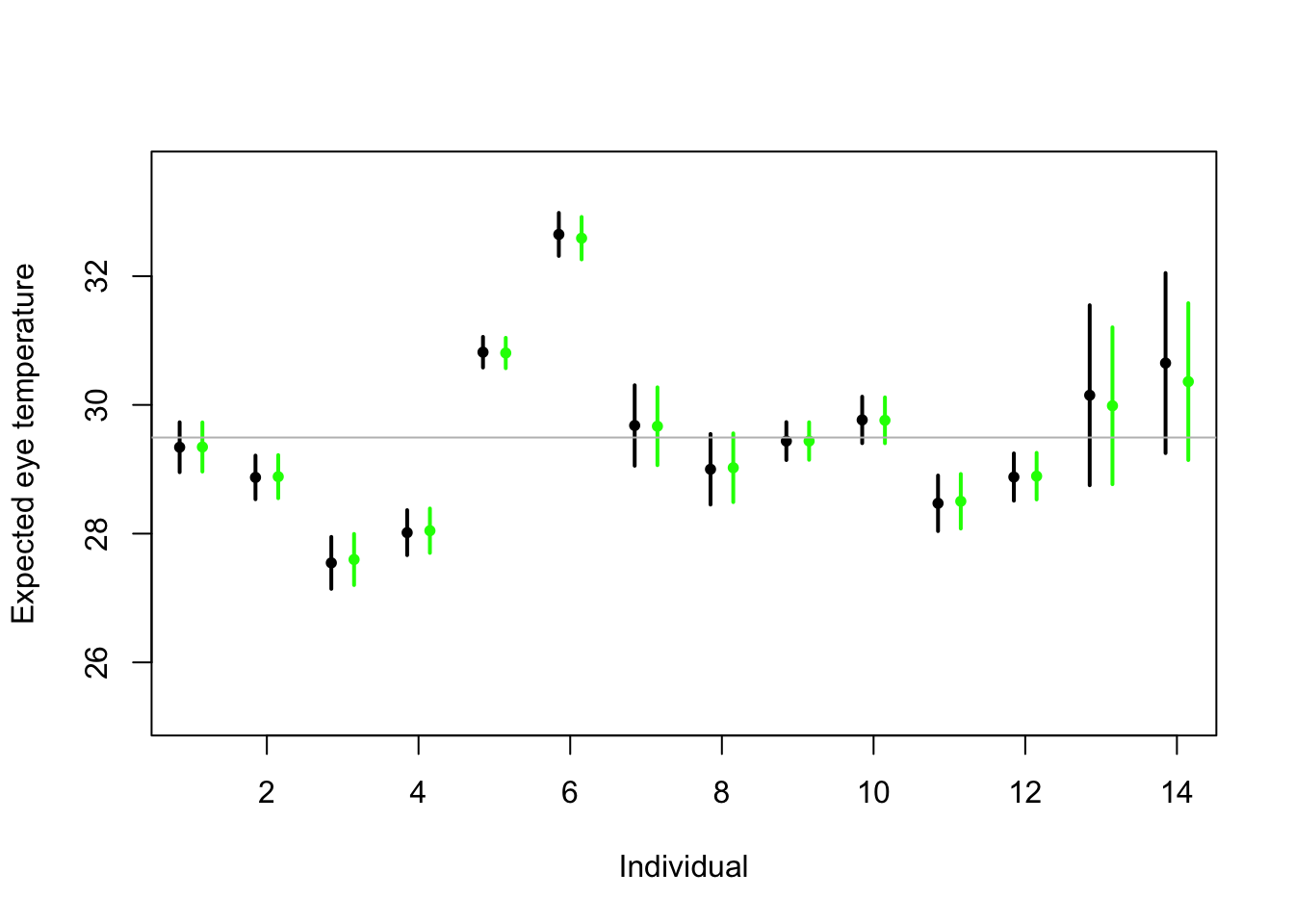
Summary
- Take home message
- Treating \(\boldsymbol{\beta}\) as a random effect “shrinks” the estimates of \(\boldsymbol{\beta}\) closer to zero.
- Requires an extra assumption \(\boldsymbol{\beta}\sim\text{N}(\mathbf{0},\sigma_{\beta}^{2}\mathbf{I})\)
- Penalty
- Random effect
- This called a prior distribution in Bayesian statistics
- Take home message
36.3 Generalized linear models
The generalized linear model framework \[\mathbf{y} \sim[\mathbf{\mathbf{y}|\boldsymbol{\mu},\psi]}\] \[g(\boldsymbol{\mu})=\mathbf{X}\boldsymbol{\beta}\]
- \([\mathbf{y}|\boldsymbol{\mu},\psi]\) is a distribution from the exponential family (e.g., normal, Poisson, binomial) with expected value \(\boldsymbol{\mu}\) and dispersion parameter \(\psi\).
- Example \([\mathbf{y}|\boldsymbol{\mu},\psi]=\text{N}\left(\boldsymbol{\mu},\psi\mathbf{I}\right)\)
- Example \([\mathbf{\mathbf{y}|\boldsymbol{\mu},\psi]}=\text{Poisson}\left(\boldsymbol{\mu}\right)\)
- Example \([\mathbf{\mathbf{y}|\boldsymbol{\mu},\psi]}=\text{gamma}\left(\boldsymbol{\mu},\psi\right)\)
- \([\mathbf{y}|\boldsymbol{\mu},\psi]\) is a distribution from the exponential family (e.g., normal, Poisson, binomial) with expected value \(\boldsymbol{\mu}\) and dispersion parameter \(\psi\).
Estimation
- Use numerical maximization to estimate
- \(\hat{\boldsymbol{\beta}}=(\mathbf{X}^{\prime}\mathbf{X})^{-1}\mathbf{X}^{\prime}\mathbf{y}\) is NOT the MLE for the glm
- Inference is based on asymptotic properties of MLE.
- Example: Challenger data
- The statistical model: \[\mathbf{y}\sim\text{binomial}(6,\mathbf{p})\] \[\text{logit}(\mathbf{p})=\mathbf{X}\boldsymbol{\beta}.\]
- The PMF for the binomial distribution \[\binom{N}{y}p^{y}(1-p)^{N-y}\]
- Write out the likelihood function \[\mathcal{L}(\boldsymbol{\beta})=\prod_{i=1}^n\binom{6}{y_i}p_i^{y_i}(1-p_i)^{6-y_i}\]
- Maximize the log-likelihood function
challenger <- read.csv("https://www.dropbox.com/s/ezxj8d48uh7lzhr/challenger.csv?dl=1")

plot(challenger$Temp,challenger$O.ring,xlab="Temperature",ylab="Number of incidents",xlim=c(10,80),ylim=c(0,6))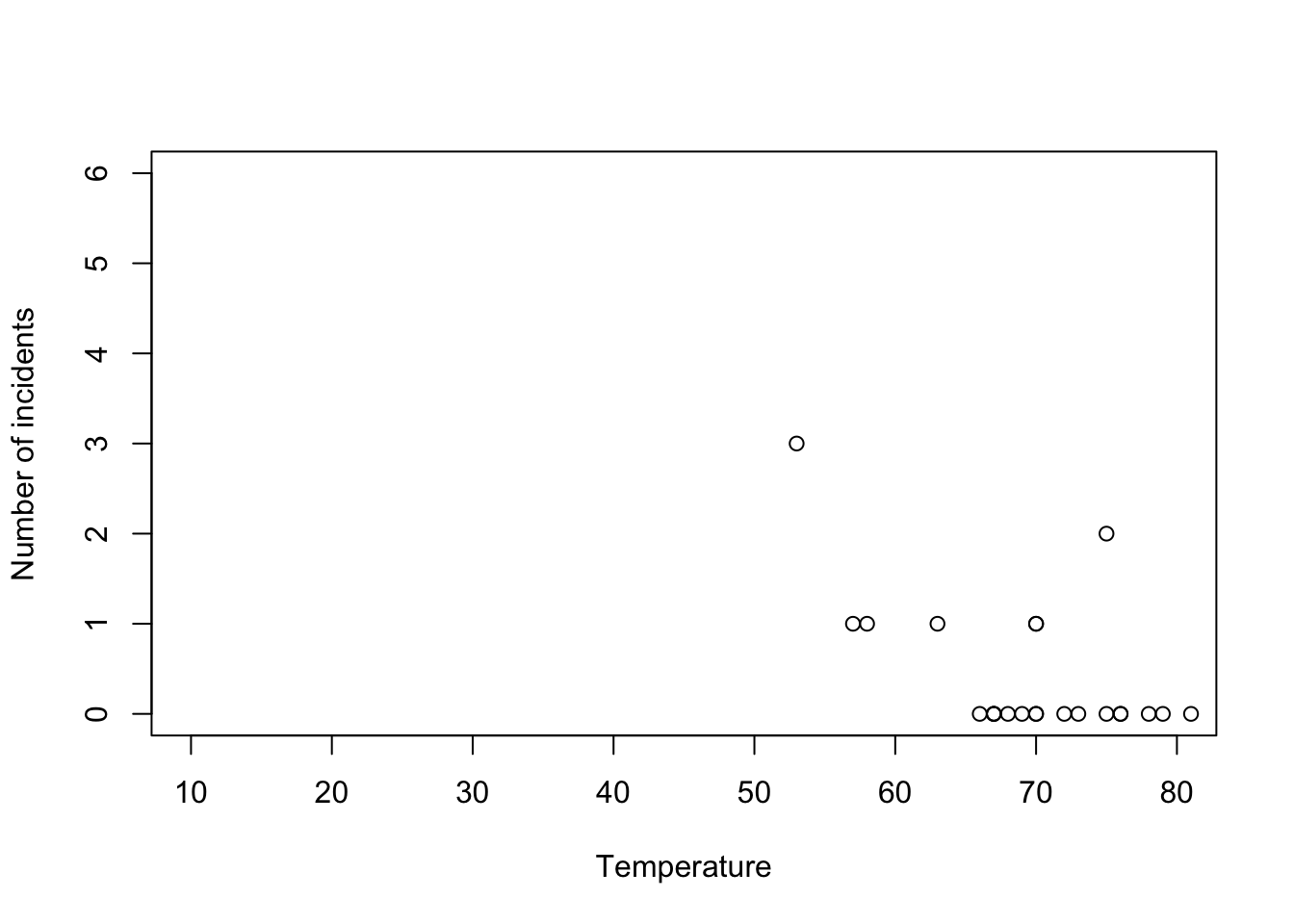
y <- challenger$O.ring
X <- model.matrix(~Temp,data= challenger)

nll <- function(beta){
  p <- 1/(1+exp(-X%*%beta)) # Inverse of logit link function
  -sum(dbinom(y,6,p,log=TRUE)) # Sum of the log likelihood for each observation
  }
est <- optim(par=c(0,0),fn=nll,hessian=TRUE)

# MLE of beta
est$par
## [1] 6.751192 -0.139703## [1] 8.830866682 0.002145791## [1] 2.97167742 0.04632268- Using the
glm()function
m1 <- glm(cbind(challenger$O.ring,6-challenger$O.ring) ~ Temp, family = binomial(link = "logit"),data=challenger)
summary(m1)
## ## Call: ## glm(formula = cbind(challenger$O.ring, 6 - challenger$O.ring) ~ ## Temp, family = binomial(link = "logit"), data = challenger) ## ## Coefficients: ## Estimate Std. Error z value Pr(>|z|) ## (Intercept) 6.75183 2.97989 2.266 0.02346 * ## Temp -0.13971 0.04647 -3.007 0.00264 ** ## --- ## Signif. codes: 0 '***' 0.001 '**' 0.01 '*' 0.05 '.' 0.1 ' ' 1 ## ## (Dispersion parameter for binomial family taken to be 1) ## ## Null deviance: 28.761 on 22 degrees of freedom ## Residual deviance: 19.093 on 21 degrees of freedom ## AIC: 36.757 ## ## Number of Fisher Scoring iterations: 5- Prediction
- We can get prediction using \(\mathbf{X}\hat{\boldsymbol{\beta}}\) or the inverse of the logit link function \(\hat{\boldsymbol{\mu}}=\frac{1}{1+e^{-\mathbf{X}\hat{\boldsymbol{\beta}}}}\)
- Confidence intervals for \(\mathbf{X}\hat{\boldsymbol{\beta}}\) are straightforward
- Confidence intervals for \(\hat{\boldsymbol{\mu}}=\frac{1}{1+e^{-\mathbf{X}\hat{\boldsymbol{\beta}}}}\) are not straightforward because of the nonlinear transformation of \(\hat{\boldsymbol{\beta}}\)
beta.hat <- coef(m1)

new.temp <- seq(0,80,by=0.01)
X.new <- model.matrix(~new.temp)

mu.hat <- (1/(1+exp(-X.new%*%beta.hat)))

plot(challenger$Temp,challenger$O.ring,xlab="Temperature",ylab="Number of incidents",xlim=c(10,80),ylim=c(0,6))
points(new.temp,6*mu.hat,typ="l",col="red")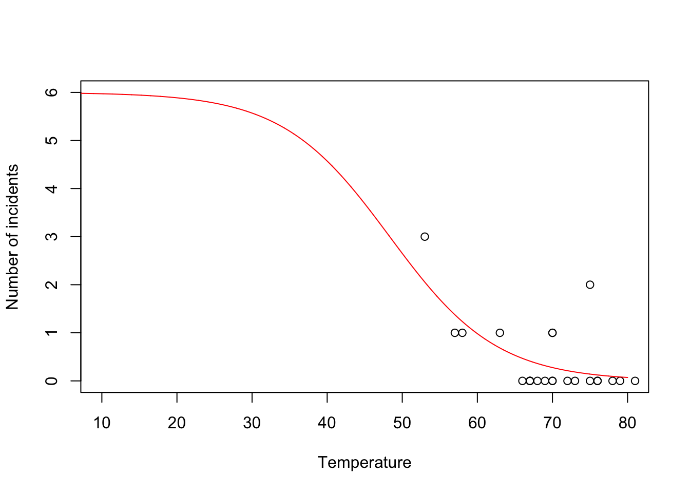
- Predictive distribution
library(mosaic)

predict.bs <- function() {
    m1 <- glm(cbind(O.ring, 6 - O.ring) ~ Temp, family = binomial(link = "logit"),
        data = resample(challenger))
    p <- predict(m1, newdata = data.frame(Temp = 31), type = "response")
    y <- rbinom(1, 6, p)
    y
}

bootstrap <- do(1000) * predict.bs()

par(mar = c(5, 4, 7, 2))
hist(bootstrap[, 1], col = "grey", xlab = "Year", main = "Empirical distribution of O-ring failures at 31 degrees",
    freq = FALSE, right = FALSE, breaks = c(-0.5:6.5))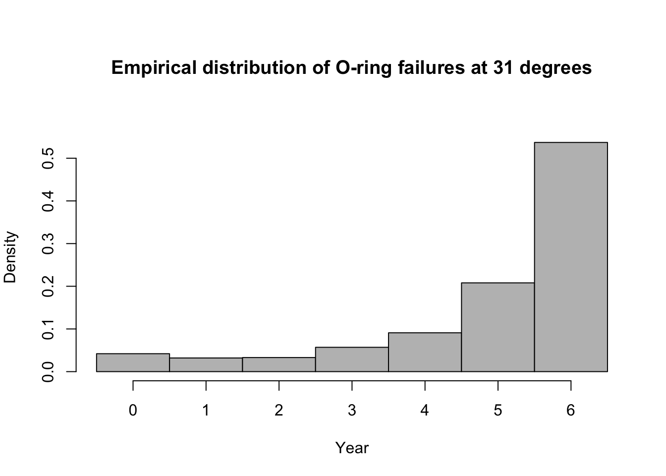
# 95% equal-tailed CI based on percentiles of the empirical distribution
quantile(bootstrap[, 1], prob = c(0.025, 0.975))
## 2.5% 97.5% ## 0 6## [1] 0.537Summary
- The generalized linear model useful when the distributional assumptions of linear model are untenable.
- Small counts
- Binary data
- Two cultures
- All distributions are approximations of a unknown data generating process so why does it matter? Use the linear model because it is easier to understand.
- Personal philosophy
- Picking a distribution whose support matches that of the data gets closer to the etiology of the process that generated the data.
- Easier for me to think scientifically about the process
- The generalized linear model useful when the distributional assumptions of linear model are untenable.