Chapter 4 Lesson 29: Analytical Solutions I

4.1 Objectives

Understand the definition of an initial value problem (IVP).
Given a pure‐time ODE, find the general solution through integration by hand.
Given an IVP, find the specific solution through integration by hand.
Describe the difference between the solution of an ODE and the solution of an IVP.

Reading

Chapter 4 of the Supplemental Reading

4.2 In class

Introduction. Over the next few lessons, we will introduce methods for solving differential equations (analytical, graphical, and numerical). To facilitate their understanding, we will start with ODEs where the right hand side is a function of the input variable (pure-time ODEs). This should be very familiar given the material thus far. After introducing these methods in this context, we will transition to more complicated ODEs later.
Direct Integration. Review basic antiderivatives from the Antidifferentiation block. Remind them that when finding the antiderivative, the result has a \(+C\) component. Remind them why this is. In this lesson, we will practice finding a particular \(C\) given an initial value/condition. This will be known as an Initial Value Problem (IVP). You may see it referred to as either a “specific” or “particular” solution, we are trying to stick with specific in this course, though the two phrases are largely interchangeable.
No Analytical Solutions. We’ll end by introducing an IVP that is not possible to solve analytically. This will segue nicely to the next lessons: graphical and numerical approximation.

R Commands

makeFun(), plotFun()

Problems & Activities

Start with review problems on ODEs and proposed solutions (the guess-and-check method). This should be done at boards or desks for the first few minutes.
Now transition to finding solutions analytically, rather than just guessing and checking. Have students find the general solution to an ODE that is integrable. (One possible example is \(y^{'} = e^{3t}\)). Find the general solution, and plot several different solutions to show the family of solutions.

If \[y'=e^{3t}\] then \[\int y'(t)\,dt = \int e^{3t}\,dt\] so \[y(t)+C_1=\frac{1}{3}e^{3t}+C_2.\] Combine the constants to get \[y=\frac13 e^{3t}+C\] where \(C=C_2-C_1.\)

Note: In the book, for a couple of examples, we carefully track the constant of integration that appears on the left-hand side of the ODE, as well as the one on the right, and then carefully combine them. However, after about two examples, we drop that practice for the more common practice of only including the constant of integration on one side of the ODE, understanding that we have already combined. Students do not need to write two constants of integration and then combine.
```
antiD(exp(3*t)~t)
```
```
## function (t, C = 0) 
## {
##     exp(3 * t)/3 + C
## }
## <environment: 0x00000291dc19f318>
```
```
y=makeFun(1/3*exp(3*t)~t)

plotFun(y(t)+0.5~t,tlim=c(-3,1),ylim=c(0,5),lwd=3,col="firebrick")
plotFun(y(t)+1~t,add=TRUE,lwd=3,col="darkorchid")
plotFun(y(t)+2~t,add=TRUE,lwd=3,col="darkgreen")
mathaxis.on()
grid.on()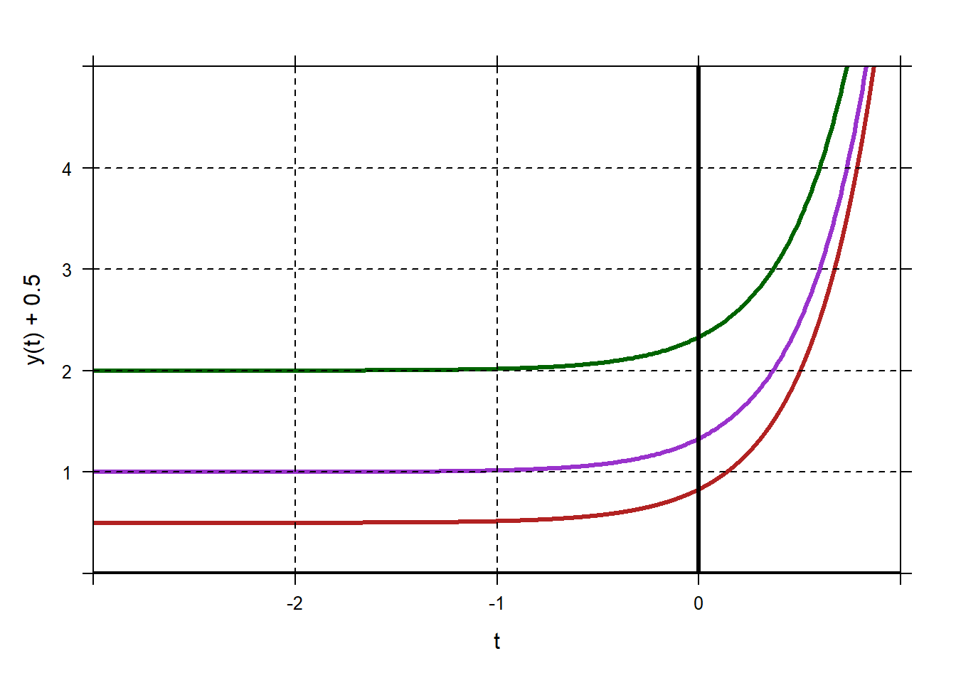
```
Now attack some initial value problems. Unlike ODEs, which have general solutions, IVPs have specific solutions. Take the ODE above, and solve it a few times with different initial conditions. \[\frac{dy}{dt}=e^{3t}\] \[\text{a) } y(0)=2\] \[\text{b) } y(1)=3\] \[\text{c) } y(2)=4\]
After wrapping up that example, cadets should spend time at board/desks on the exercises at the end of the reading.
End class with an example that is not possible to integrate “by hand”, such as the one in the reading: \(y^{'} = e^{- t\sqrt{t}}\). Note that we will have to explore other methods to analyze this equation.