Chapter 12 Lesson 37: Systems of ODEs II

12.1 Objectives

Given a system of two first‐order ODEs, find all equilibrium solutions of the system algebraically by hand or using R.
Given a phase plane for a system of two first‐order ODEs, sketch a specific solution given an initial condition, visually identify any equilibrium solutions and determine the stability of each equilibrium (stable or unstable).
Visually match a system of two first‐order ODEs to its corresponding phase plane.
Use R to produce a phase plane for a given system of two first‐order ODEs.

The official course objectives say that students should be able to find equilibrium solutions by hand. That is a typo. It is fine if they use findZeros.
The objectives say they should be able to visually match a system of ODEs to the phase plane. This is very similar to this example from direction fields, as well as exercises 5-12 from Exercises 5.3. If you have time, do a few of these, there are problems at the end of the chapter. However, I’m pretty comfortable asking the cadets to do it on their own.

Do one warm up problem of finding an equilibrium solution to a system of ODEs. Pick any example from the text that you haven’t used yet.
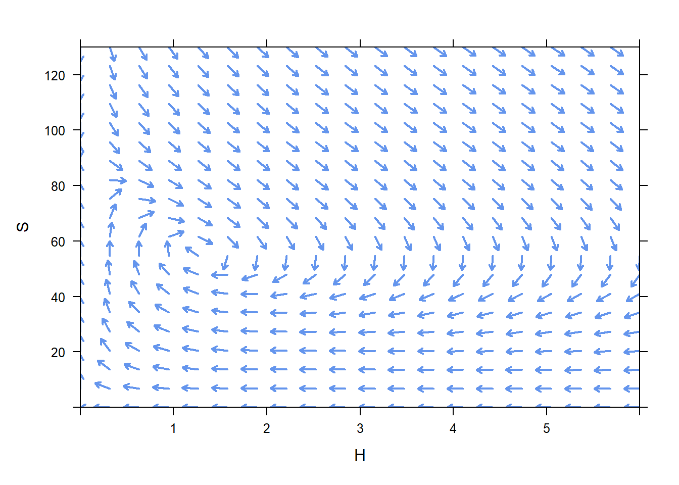
Now start sketching a phase plane. Follow the development in the book. Each point in the plane is used to represent a possible state (in the book, populations). From each potential state that we could reach, we ask the ODE how the population would change from here. Then we draw a vector heading in the direction the ODE prescribed. This would be a good exercise to do on the board.
Once you’ve done a few vectors in the phase plane, use plotPhasePlane to get the full picture.
Talk about the difference between phase planes and direction fields. They look a lot the same, they are used to do the same thing. However, there is no time axis on a phase plane. You can indeed “follow the flow” on a phase plane to get an approximate solution to an IVP, but you won’t be able to read off the phase plane the time at which the solutions achieve each state.
Finally, stability. Follow the books lead and use examples with physical interpretations. Interpret the stability of an equilibrium solution as “If the initial condition changes from the equilibrium initial condition by a little, the solution to the IVP will/won’t change a lot”.

findZeros, plotPhasePlane

After a warmup of finding an equilibrium solution, develop the notion of the phase plane. It is much like the phase line, but since there are two quantities changing we need two axes, thus the phase plane. Follow the development in the book.
Once you’ve drawn a few vectors on the board, use plotPhasePlane to help you along.

plotPhasePlane(c(-0.5*H+0.009*S*H, 
                  0.3*S*(1-S/90) - 0.09*S*H)~H&S,
               xlim=c(0,6),ylim=c(0,130))

Once you have a phase plane in mind, ask how the populations might evolve if the initially start at \(H=3\), \(S=100\)? Just like a direction field, the solution will “flow along” the arrows. This is a place where I would project the phase plane on the board, draw a big dot at position \(H=3\), \(S=100\), and then have them tell me how to flow along the directions.
Now, interpret this curve you have drawn. The curve passes through several points, for example \(H=4.26\), \(S=55.32\). That means that at some time we expect there to be 4.26 hawks and 55.32 squirrels living in the park. Interpret a few other points. Have the students describe in words how this population behaves. Something like “Initially, the number of hawks in the park increases, while the number of squirrels decreases. Once the population reaches roughly 4.25 hawks and 50 squirrels, though, the number of hawks starts decreasing (they are running out of squirrels to eat), and while the number of squirrels continues to decline. Once the population reaches about 2 hawks and 30 squirrels, the number of squirrels start to rebound (there aren’t as many hawks to eat them), while the hawk population continues declining”, and so on.
You can actually draw the curve you sketched on the board by giving plotPhasePlane an initial condition to start from.

plotPhasePlane(c(-0.5*H+0.009*S*H, 
                  0.3*S*(1-S/90) - 0.09*S*H)~H&S,
               xlim=c(0,6),ylim=c(0,130),ics=c(3,100))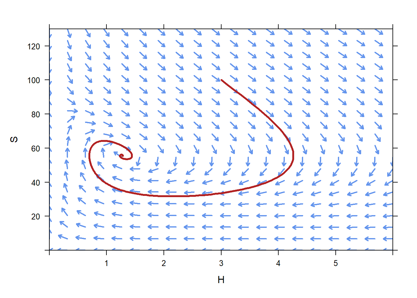

Finally, interpret that point in the center of the swirl. It is an equilibrium solution!
Now, ask what would happen if the initial condition were not exactly on the equilibrium solution. This one is a little hard to tell, but it looks like no matter where you start, the populations will eventually swirl in to the equilibrium state. That makes it a stable equilibrium solution.
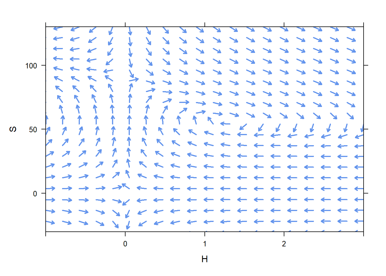
Consider the other equilibrium solutions by plotting a the phase plane over a bigger window, as done in the book. Ask them to visually identify the equilibrium solutions, and ask them to visually classify the stability of the equilibrium solutions.

plotPhasePlane(c(-0.5*H+0.009*S*H,0.3*S*(1-S/90)-0.09*S*H)~H&S,
               xlim=c(-1,3),ylim=c(-30,130))

As time allows, pursue some more examples. They might especially like Lanchester’s Laws, or the Pendulum Example