Chapter 2 Notes about USAFACalc Relevant to Block 6
In Block 6 we follow the Supplemental Reading available online here. All of the R functionality that we need for this block has now been built into USAFACalc. It is a good idea to run updateUSAFACalc before you begin the block, as there have been several minor convenience changes, and one actual bug fix, since the students created their projects.
Below find the R commands we’ll be using in class. These all have reasonable documentation, you can find documentation and examples by using the ? operator, for example ?plotODEDirectionField.
Students should be able to use plotODEDirectionField, Euler, and plotPhasePlane for the homework, GR, and/or final exam. They’ll use animateODESolution for the project, but that’s it.
2.1 plotODEDirectionField
plotODEDirectionField Plots the direction field for a scalar ODE. Direction field, not slope field (direction fields have normalized vectors). There is no command for plotting slope fields, although you could certainly use plotVectorField to achieve it by defining the vector-valued function \((1,f(t,y))\).
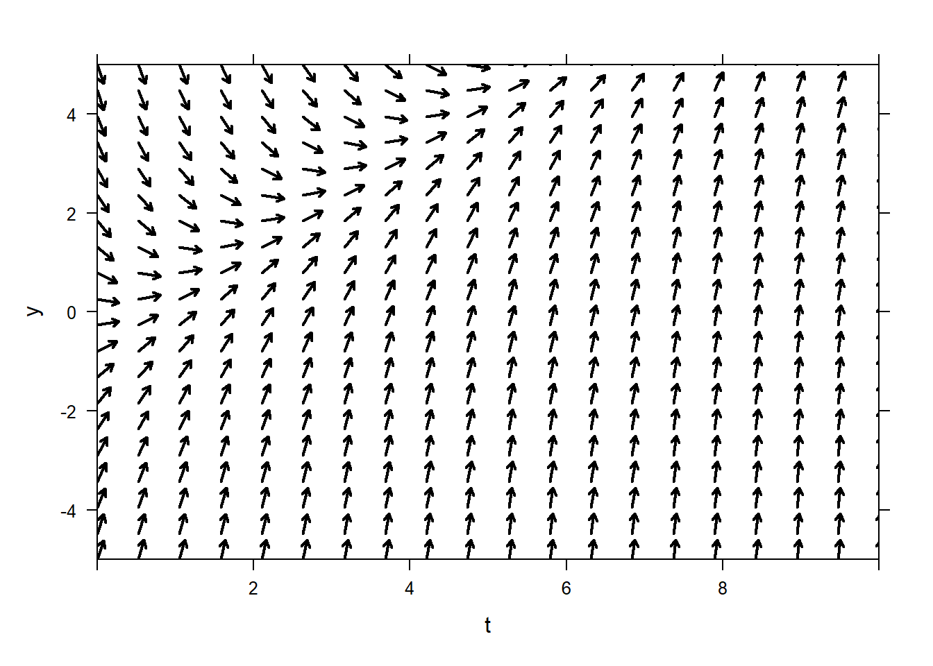
In general, the R ODE functions only require the right-hand side of first-order ODEs. So to plot a direction field for the ODE
\[y'=t-y\]
use the following, note that we are only giving it the right-hand side. In general the right-hand side ODEs need to be functions of \(t\) and \(y\), in that order. Don’t reverse \(t\) and \(y\), and don’t omit either of them, even if one of them doesn’t show up in the ODE.
 You can vary the arrow thickness and color using
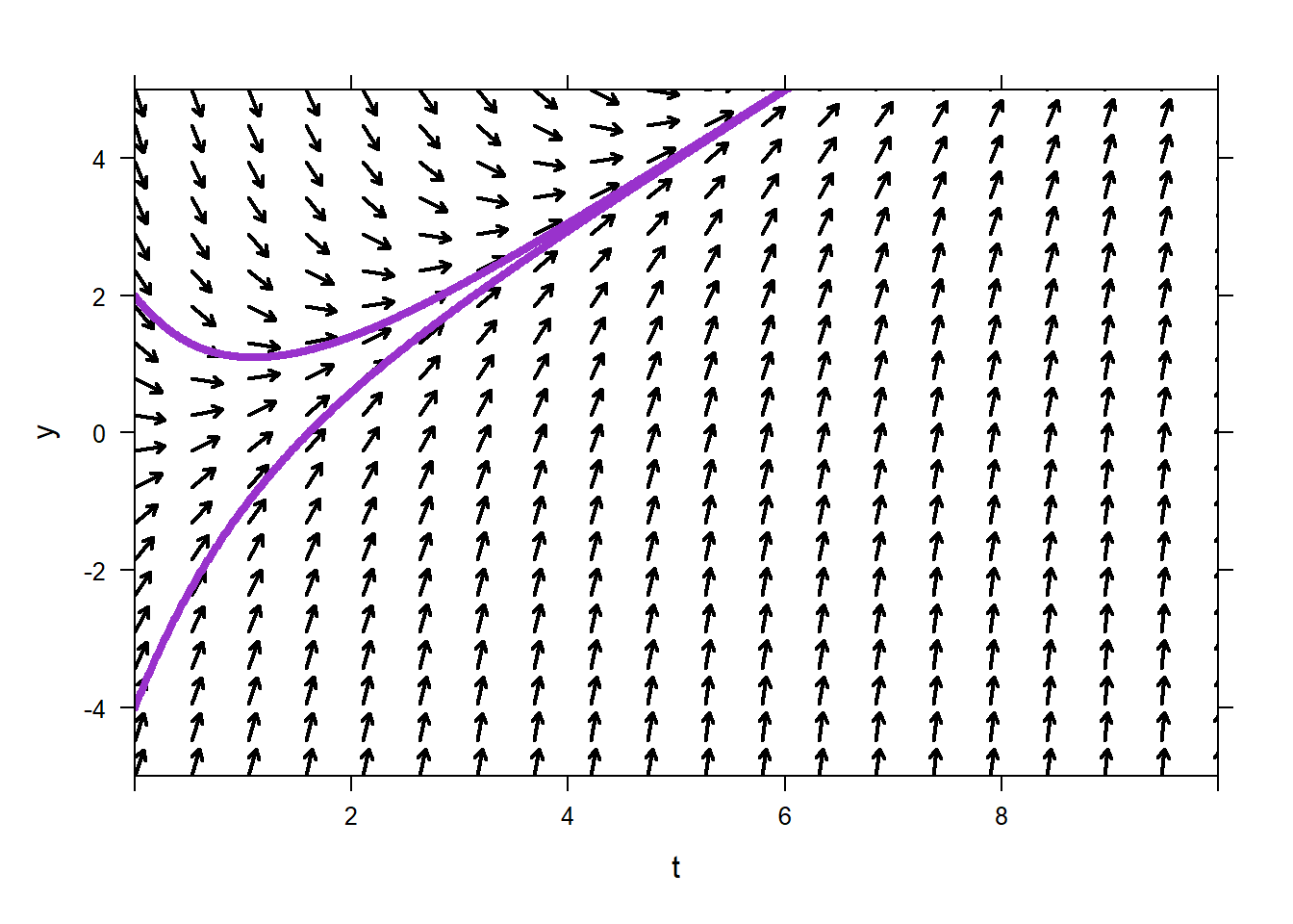
 lwd and col, as usual. You can plot trajectories that correspond to initial conditions as follows. You can plot one or many trajectories. It is assumed that the initial condition always occurs on the left-hand side of the figure, so you only need to give the \(y\)-value of the initial condition(s).
plotODEDirectionField(t-y~t&y,tlim=c(0,10),ylim=c(-5,5),ics=2)
plotODEDirectionField(t-y~t&y,tlim=c(0,10),ylim=c(-5,5),ics=c(2,-4))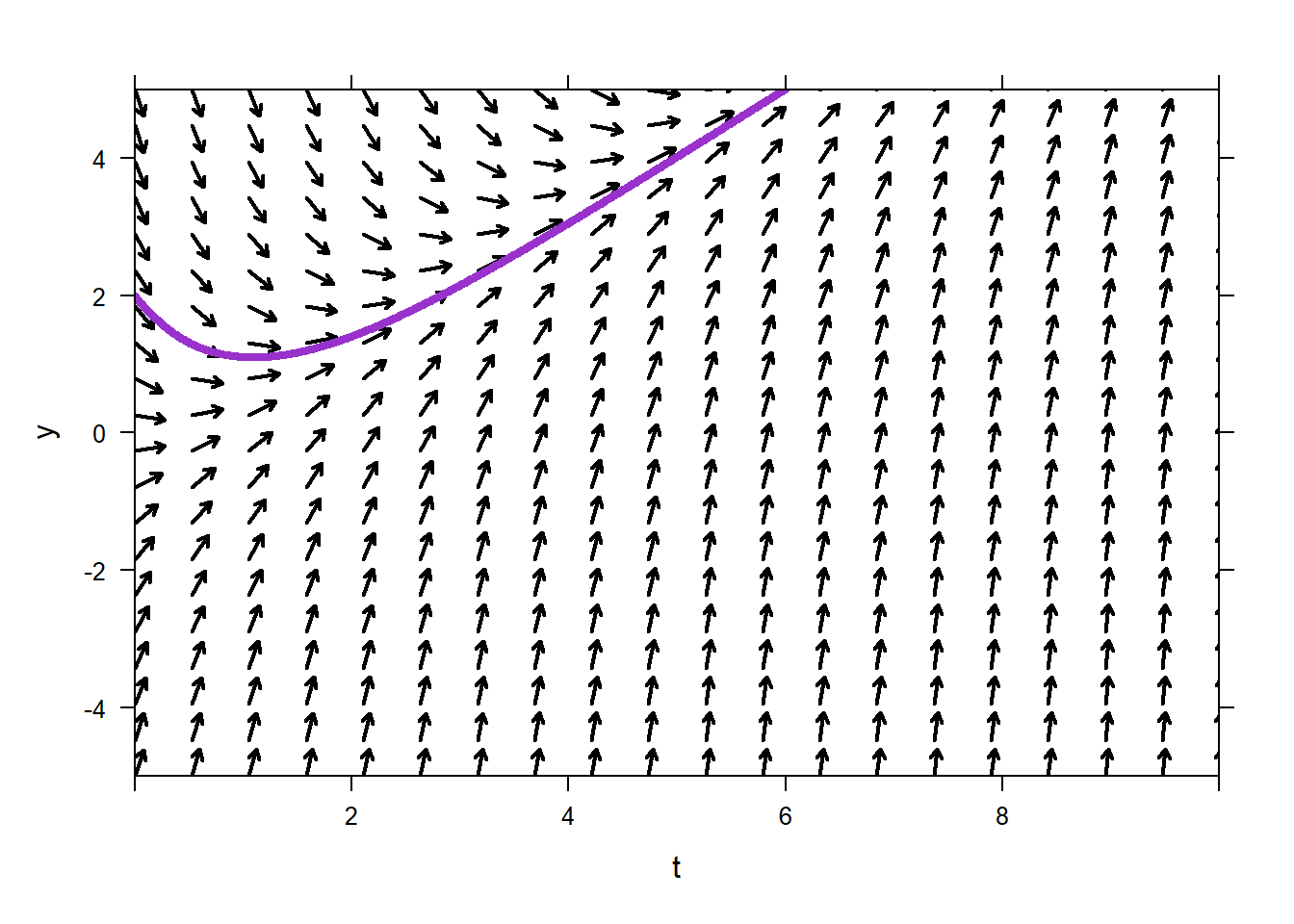
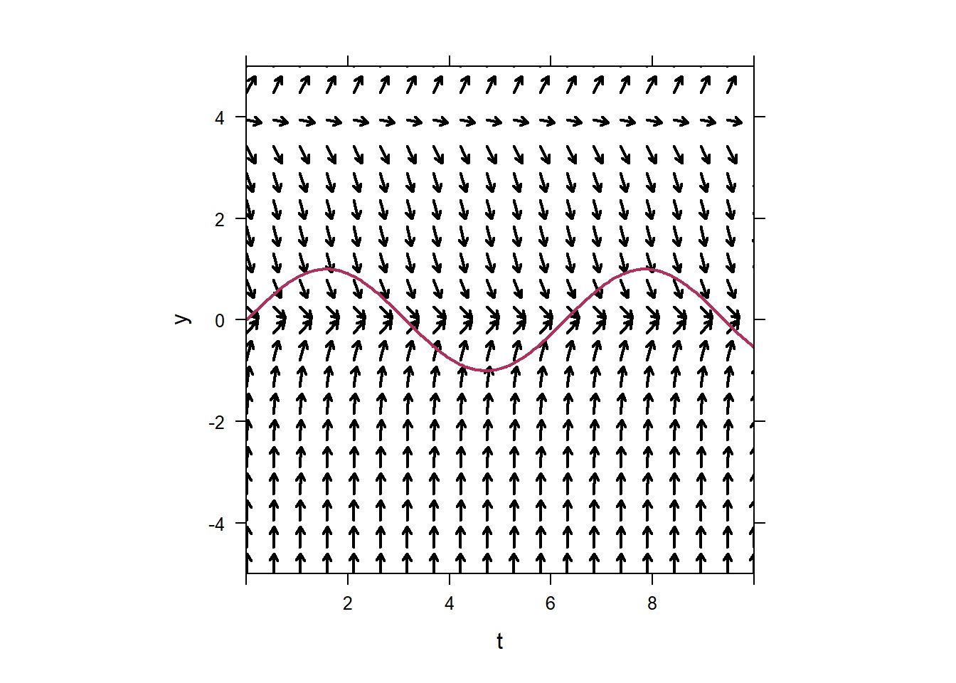
plotODEDirectionField works fine with the add option, or other things can be added to a direction field, so you can overlay plots of whatever function you like on top of the direction field. For instance a solution to the ODE, or a not-the-solution to the ODE.
Consider the ODE
\[y'=y(y-4).\]
Note how there is no \(t\)-dependence on the right-hand side of the ODE. With plotODEDirectionField you can omit the \(t\) variable. You can not omit the \(y\) variable if the ODE is \(y'=t(t-4)\). It is safest to always declare the right-hand side to be a function of \(t\) and \(y\).
Sometimes your direction field will look weird because the aspect ratio is not 1:1 by default. If your vertical arrows look short, but horizontal ones look long, the aspect ratio your problem. You can set asp=1 to fix this.
2.2 Euler
Euler performs Euler’s method on a given first-order ODE. The goal is that students should be able to do Euler’s method by hand, but when it comes time to do it for lots of iterations then obviously we’ll just use the computer.
The syntax is very similar to plotODEDirectionField. Specify the right-hand side of the ODE, give the time interval you are interested in and the value of the initial condition, and optionally set the step size. You do not need to stick to \(y\) as the unknown function, you can name it what you like.
##      t         P
## 1  0.0 0.1000000
## 2  0.1 0.1490000
## 3  0.2 0.2212799
## 4  0.3 0.3270234
## 5  0.4 0.4798406
## 6  0.5 0.6967362
## 7  0.6 0.9965602
## 8  0.7 1.3955271
## 9  0.8 1.8985411
## 10 0.9 2.4873658
## 11 1.0 3.1123498
2.2.1 Fancier Euler
The command Euler has had some extra work put into it. It will let you specify the ODE as an equality, in standard form, so long as you use “_t” to denote derivative. For example, the IVP
\[P'=P(5-P),\quad P(0)=0.1\]
could be approximated with
##      t         P
## 1  0.0 0.1000000
## 2  0.1 0.1490000
## 3  0.2 0.2212799
## 4  0.3 0.3270234
## 5  0.4 0.4798406
## 6  0.5 0.6967362
## 7  0.6 0.9965602
## 8  0.7 1.3955271
## 9  0.8 1.8985411
## 10 0.9 2.4873658
## 11 1.0 3.1123498
Allowing the specification of the entire equation will help with clarity later on.
2.2.2 Euler’s Method for Systems of ODE
Our Euler’s method can approximately solve arbitrarily large systems of ODEs. To solve the system of equations
\[\begin{aligned}
&x'=-y&\quad x(0)=1\\
&y'=x&\quad y(0)=0.5\\
\end{aligned}\]
We can use a syntax very much like findZeros, where we just specify the right-hand side of the ODE, specified as a vector-valued function.
##      t          x          y
## 1  0.0  1.0000000  0.5000000
## 2  0.5  0.7500000  1.0000000
## 3  1.0  0.2500000  1.3750000
## 4  1.5 -0.4375000  1.5000000
## 5  2.0 -1.1875000  1.2812500
## 6  2.5 -1.8281250  0.6875000
## 7  3.0 -2.1718750 -0.2265625
## 8  3.5 -2.0585938 -1.3125000
## 9  4.0 -1.4023438 -2.3417969
## 10 4.5 -0.2314453 -3.0429688
## 11 5.0  1.2900391 -3.1586914
This works, however, the order of the variable declaration is very important. It is assumed that because \(x\) is the first variable in t&x&y, that the first function in c(-y,x) is the derivative of \(x\), and that the first value in c(1,0.5) is the initial value of \(x\). This is easy to mess up.
It is better to use the option to specify the entire equation with Euler in this case.
##      t          x          y
## 1  0.0  1.0000000  0.5000000
## 2  0.5  0.7500000  1.0000000
## 3  1.0  0.2500000  1.3750000
## 4  1.5 -0.4375000  1.5000000
## 5  2.0 -1.1875000  1.2812500
## 6  2.5 -1.8281250  0.6875000
## 7  3.0 -2.1718750 -0.2265625
## 8  3.5 -2.0585938 -1.3125000
## 9  4.0 -1.4023438 -2.3417969
## 10 4.5 -0.2314453 -3.0429688
## 11 5.0  1.2900391 -3.1586914
Now everything is unambiguous, you can mess up the order of things as much as you like.
2.3 plotPhasePlane
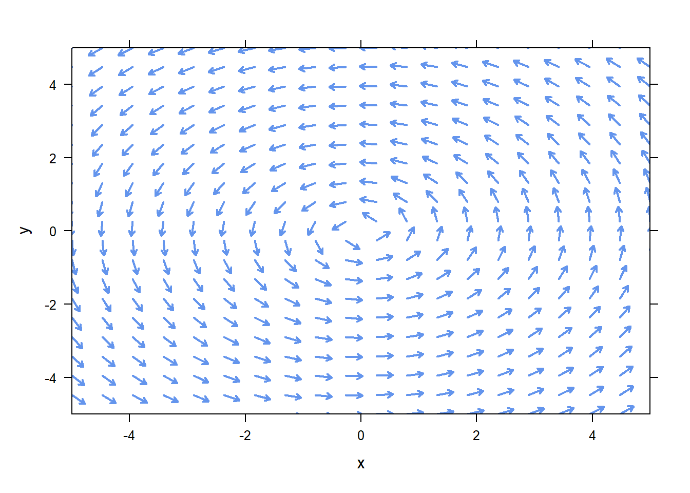
For systems of two autonomous ODEs we have plotPhasePlane, which works very much like plotODEDirectionField.
For the system of ODE \[\begin{aligned} &x'=-y\\ &y'=x\\ \end{aligned}\] we can plot the phase plane as below.
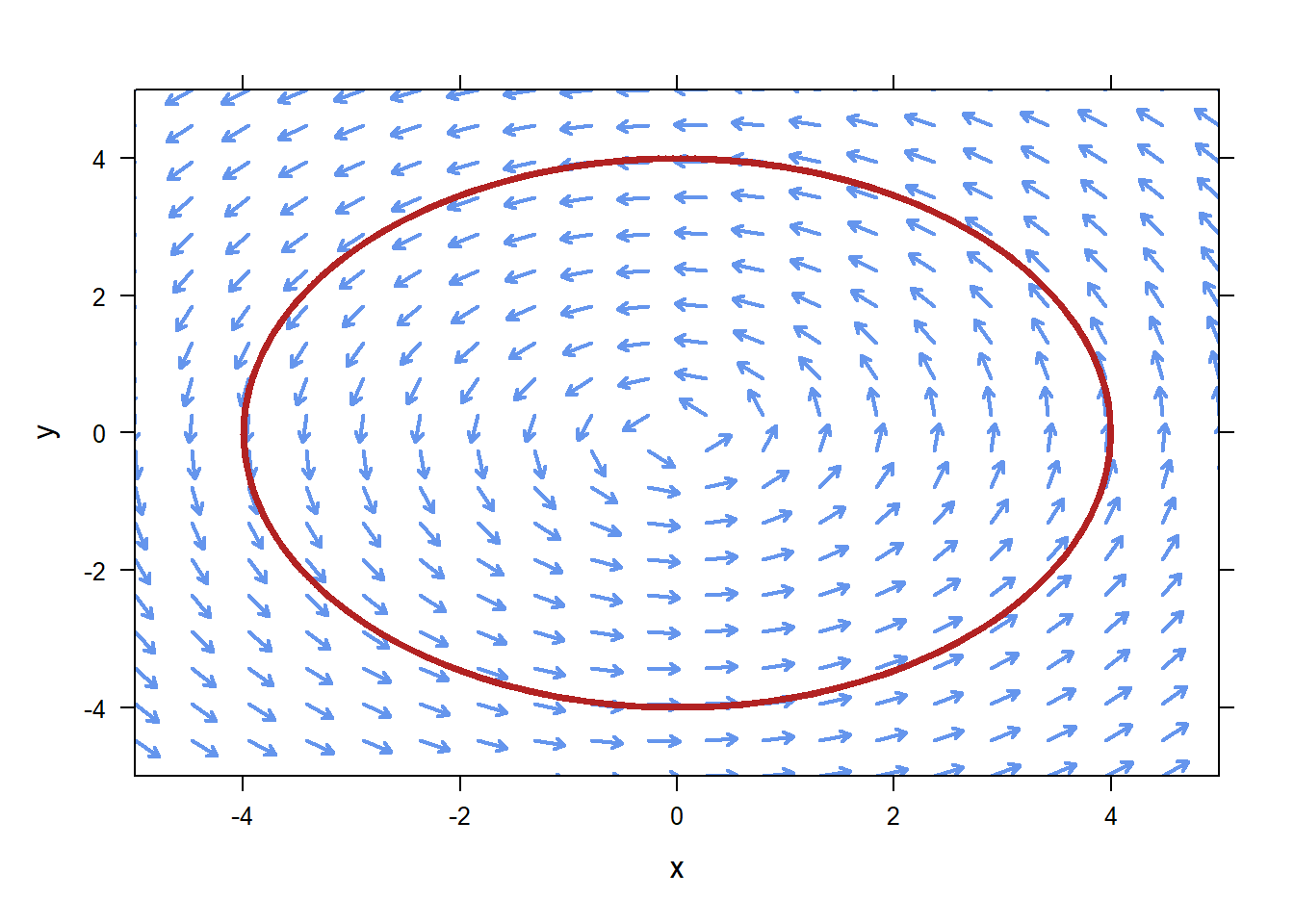
plotPhasePlane also allows you to add trajectories to your phase plane. If you wish to plot the trajectory associated with the initial condition \(x(0)=0\), \(y(0)=-2\), use the code
 If you want to specify multiple initial conditions, you must put them in a
 list.
plotPhasePlane works fine with the usual add argument, so you can add a plot of an arbitrary function or whatever you like on this. However, remember that for a phase plane you most likely want a parameteric equation. For example, one solution to the system above is
\[x(t)=\cos(t)\]
\[y(t)=\sin(t).\]
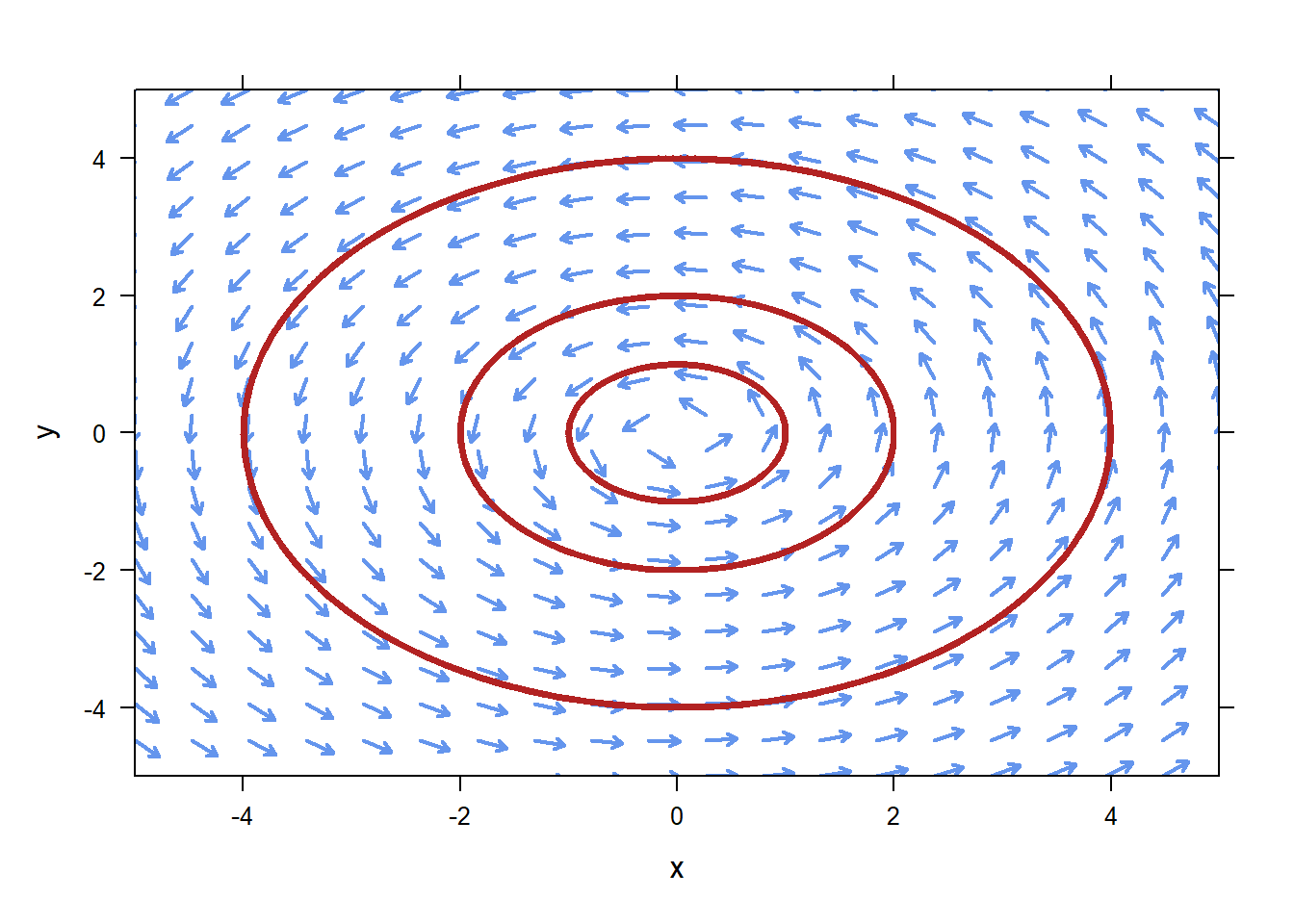
To plot the trajectory on the phase portrait, you’ll need to evaluate \(x\) and \(y\) at a large number of \(t\)-values, and then plot the \(x-y\) pairs. To do that, you’ll want to use plotPoints, likely with the optional argument type="l" to make it connect your points with a line. Example:

#Define my x(t), y(t)
x=makeFun(cos(t)~t)
y=makeFun(sin(t)~t)
ts=seq(0,2*pi,by=0.1)
plotPoints(y(ts)~x(ts),add=TRUE,type="l",col="firebrick",lwd=3)
2.4 animateODESolution
Phase planes with trajectories on them are great, but it is hard to see how the solution changes in time. We can animate the solution to our ODE using animateODESolution. To use it, first approximate a solution to the system (or scalar) equation using Euler. Then, tell animateODESolution what relationship you’d like to animate. For instance, to see how the \(x\)/\(y\) coordinates change, i.e., how the particle moves, for this IVP:
\[\begin{aligned} &x'=-y&\quad x(0)=1\\ &y'=x&\quad y(0)=0.5\\ \end{aligned}\]
we can do this:
soln=Euler(c(x_t=-y,y_t=x)~t&x&y,tlim=c(0,10),ic=c(x=0,y=3),stepSize=0.01)
animateODESolution(y~x,data=soln)
If you are interested the \(x\) and \(y\) coordinates versus time, you could do
soln=Euler(c(x_t=-y,y_t=x)~t&x&y,tlim=c(0,10),ic=c(x=0,y=3),stepSize=0.01)
animateODESolution(y~t,x~t,data=soln)
animateODESolution will show up on Project 3, but it is mostly a novelty. It’s hard to get anything quantitative out of these animations. They just look nice and make student’s say “ooh”.