Chapter 5 Lesson 30: Graphical Solutions

5.1 Objectives

Given a first‐order ODE, plot a subset of vectors from its slope field by hand.
Describe the difference between a slope field and a direction field.
Given a first‐order ODE, use R to plot a corresponding direction field.
Given a direction field for an ODE and an initial condition, sketch the corresponding specific solution.
Visually match a first‐order ODE to its corresponding direction field, including which are pure‐time and which are autonomous.

5.2 Reading

Chapter 5 of the Supplemental Reading Material

5.3 In class

Visualizing ODEs. In this lesson, we’ll introduce methods to visualize first-order ODEs. Visualization is often helpful when dealing with ODEs that don’t have analytical solutions.
Vector Fields. We’ll discuss two types of vector fields – slope fields and direction fields. The only difference between the two is that slope fields show vectors of differing lengths, while direction fields normalize the magnitude of every vector; the only thing you pay attention to in a direction field is the direction the vector heads. Sometimes the vector magnitudes are too large or small which make the graph of a slope field difficult to read; however, the corresponding direction field graph should be legible (this is why we will be mainly focused on creating and using direction fields). We are going to define the slope field vectors to be \((1,f(t,y))^T\), where \(f(t,y)\) is the right-hand side of the ODE. Obviously there are other ways to define a vector with slope \(f(t,y)\), but that definition is common for slope fields.
Direction Fields in R USAFACalc offers plotODEDirectionField. Use that in class.

5.4 R Commands

plotODEDirectionField

Problems & Activities

Start with a first-order ODE \(y^{'} = t^{2}\). Draw or project a grid on the board (or paper) and ask the students to draw the vectors that occur at various input values. If you want to produce slides with pre-drawn vectors, use the place.vector command, documented in Block 5 NTIs.

Since we are not going to get into how to normalize a vector in this course, this exercise is actually drawing vectors for a slope field. I like to think of it like this: there are infintely many solutions to my ODE. I have no idea of a formula for any of them. However, I know that if the graph of one of the solutions happens to pass through \((t=1,y=0)\), then the ODE tells me that the slope of that solution must be \(y'(1)=1^2=1\). So I’ll draw a vector with slope 1 at the point \((t=1,y=0)\), showing that if a solution passes through this point, it must be headed in this direction.

Some \((t,y)\) input values you could use include (1,0), (1,1), (1,-1), (0,1), (-1,0).
You (or they) may wonder why the axis for the vectors fields are \(t\) and \(y\). We are not actually graphing \(y(t)\), instead we are graphing a snapshot of what what a solution to the ODE must do (i.e. the slope of its graph), if it passes through the vectors base points.
Use plotODEDirectionField to create the direction field for the ODE.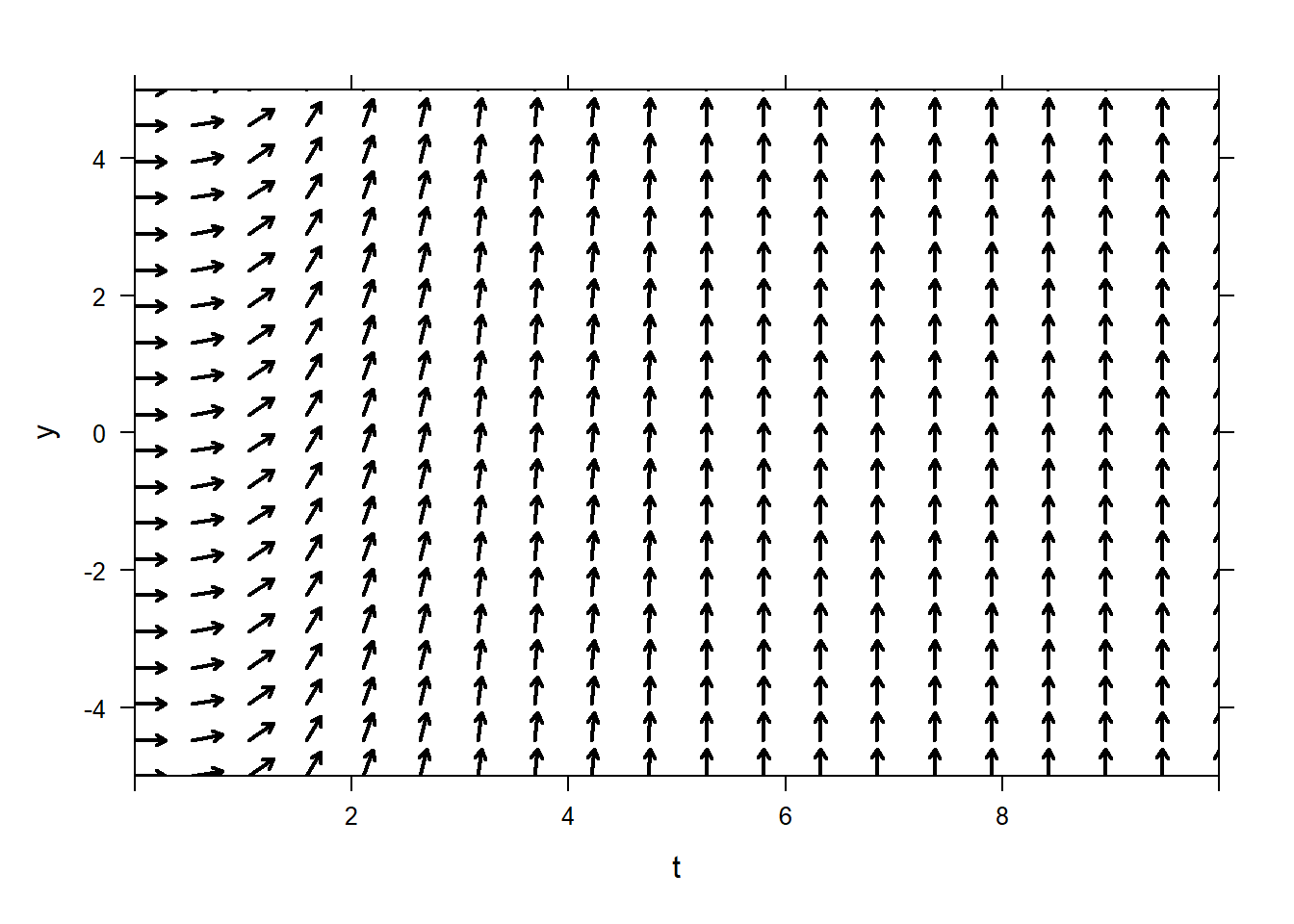
```
  plotODEDirectionField(t^2~t&y)
```
when using plotODEDirectionField, you only specify the right-hand side of the ODE. plotODEDirectionField is very general, but as a result you need to make sure your right-hand side is defined as a function of both \(t\) and \(y\), in that order.

The syntax of plotODEDirectionField should be very familiar by now. Adjust the \(t\)-axis with tlim=. Adjust the \(y\)-axis with ylim=. Adjust the color with col=.
Now, pick an initial condition, e.g., \(y(0) = 2\), and use the direction field to sketch the solution by hand. Since you know that the vectors tell you the slope of the tangent line of the graph of the solution, you just “follow the arrows”. This is a lot like dropping a volleyball into a river (vector field) and watching the path (solution) taken by the volleyball. The spot where the volleyball first lands in the river is the “initial condition.”
Show them how to get R to plot the solutions for you using the ic= option. Watch out, it is assumed that the initial condition is specified at the left-hand side of the graph, so if you want a solution corresponding to initial condition \(y(0)=2\), then you’ll need to make your tlim start at time 0.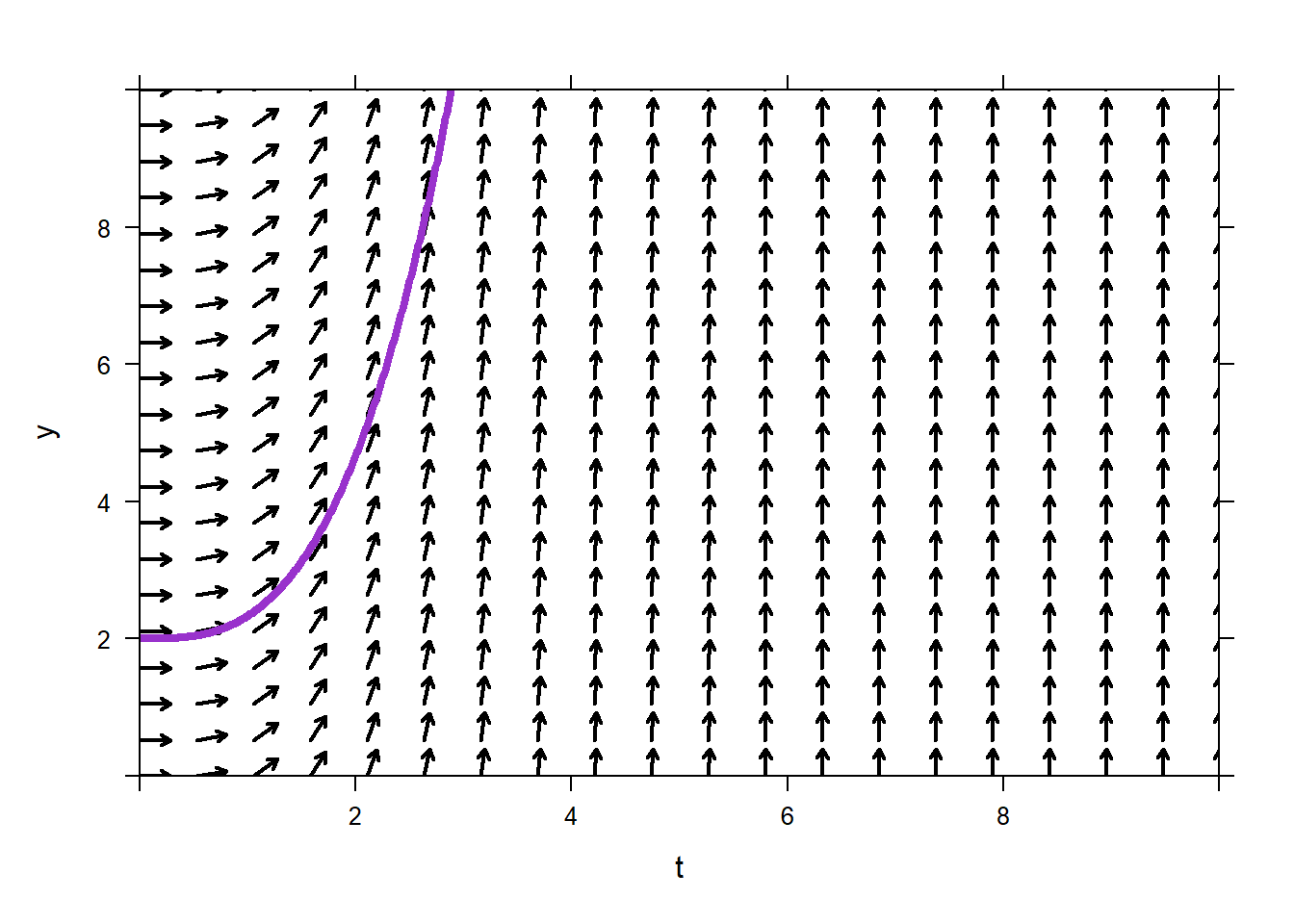
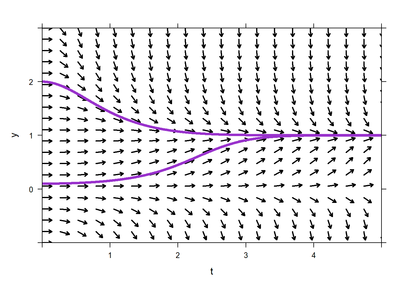
```
  plotODEDirectionField(t^2~t&y,tlim=c(0,10),ylim=c(0,10),ic=2)
```
Repeat the exercise: sketch a few vectors by hand, then make a direction field using R, then sketch a specific solution corresponding to an initial condition, then use R to sketch the solution corresponding to the initial condition, for another ODE, this one should have \(y\) on the right-hand side of the ODE. For example, something like: \[y'=ty(1-y)\] \[y(0)=0.1\] \[y(0)=2\] The only difference now is that in order to evaluate \(y'\), you’ll need to involve the \(y\)-coordinate of the base points of your vectors. Otherwise, it is exactly the same.
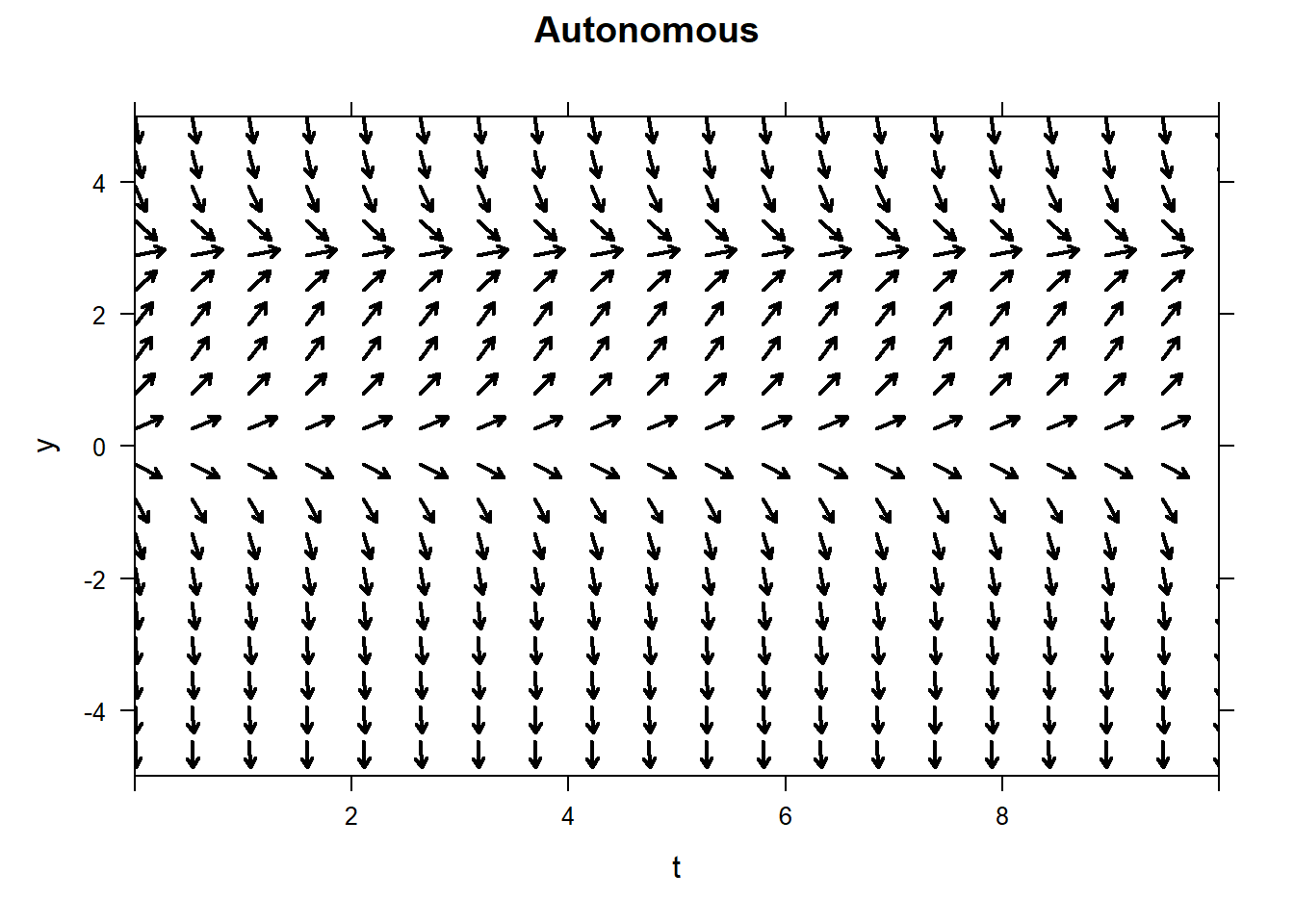
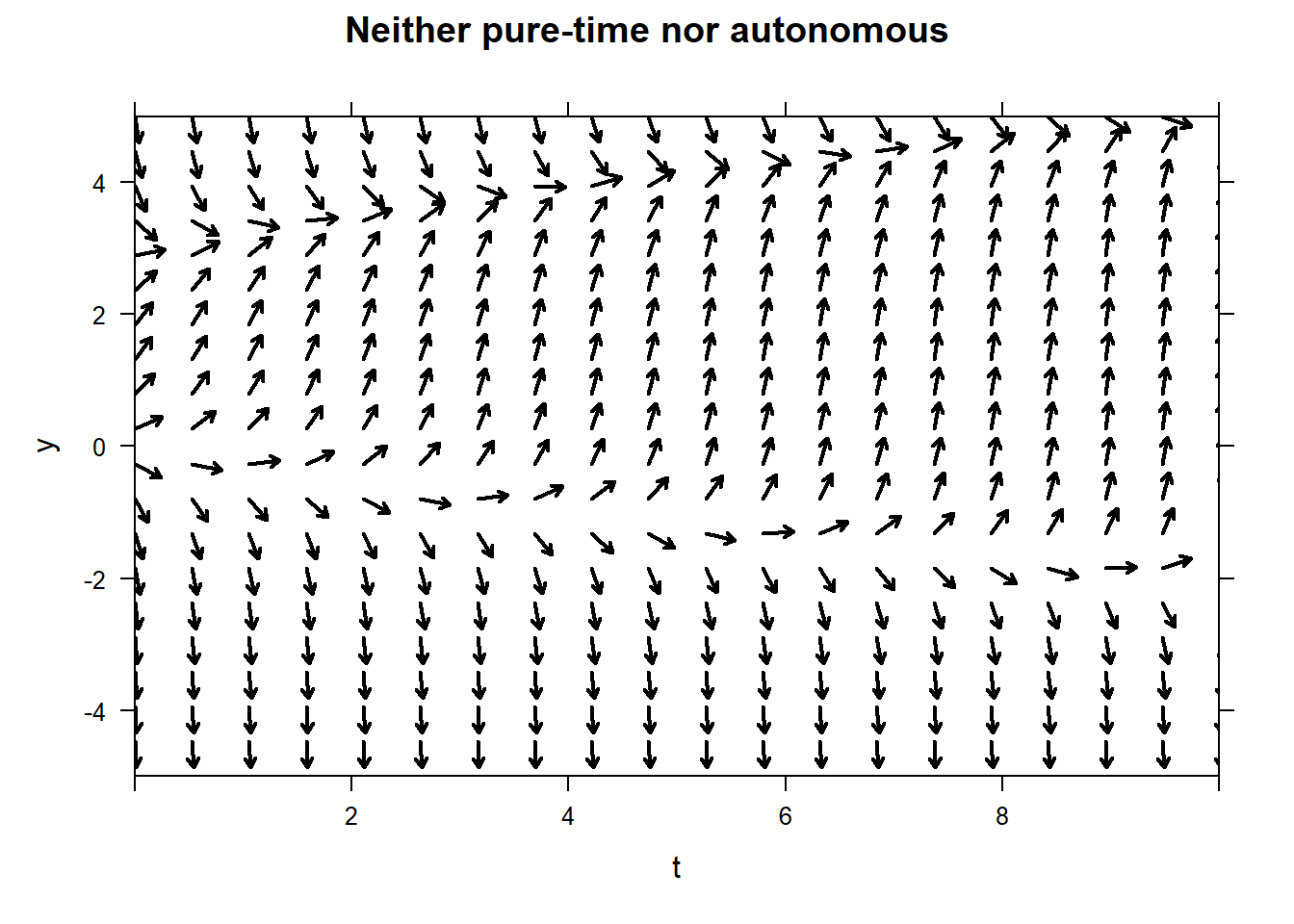
```
plotODEDirectionField(t*y*(1-y)~t&y,tlim=c(0,5),ylim=c(-1,3),ics=c(0.1,2))
```
Talk about the difference between pure-time and autonomous differential equations. In a pure-time ODE, the right hand side only depends on \(t\). We saw how to solve some of those yesterday. In an autonomous ODE, the right-hand side only explicitly depends on \(y\). The direction fields for those will look different. For a pure-time ODE, the direction field will have vectors that do not change in the \(y\)-direction. The autonomous direction field will have vectors that do not change in the \(t\)-direction.

    #pure-time
    plotODEDirectionField(sin(t)~t&y,main="Pure-Time")

    #autonomous
    plotODEDirectionField(y*(3-y)~t&y,main="Autonomous")

    #Niether
    plotODEDirectionField(y*(3-y)+t~t&y,main="Neither pure-time nor autonomous")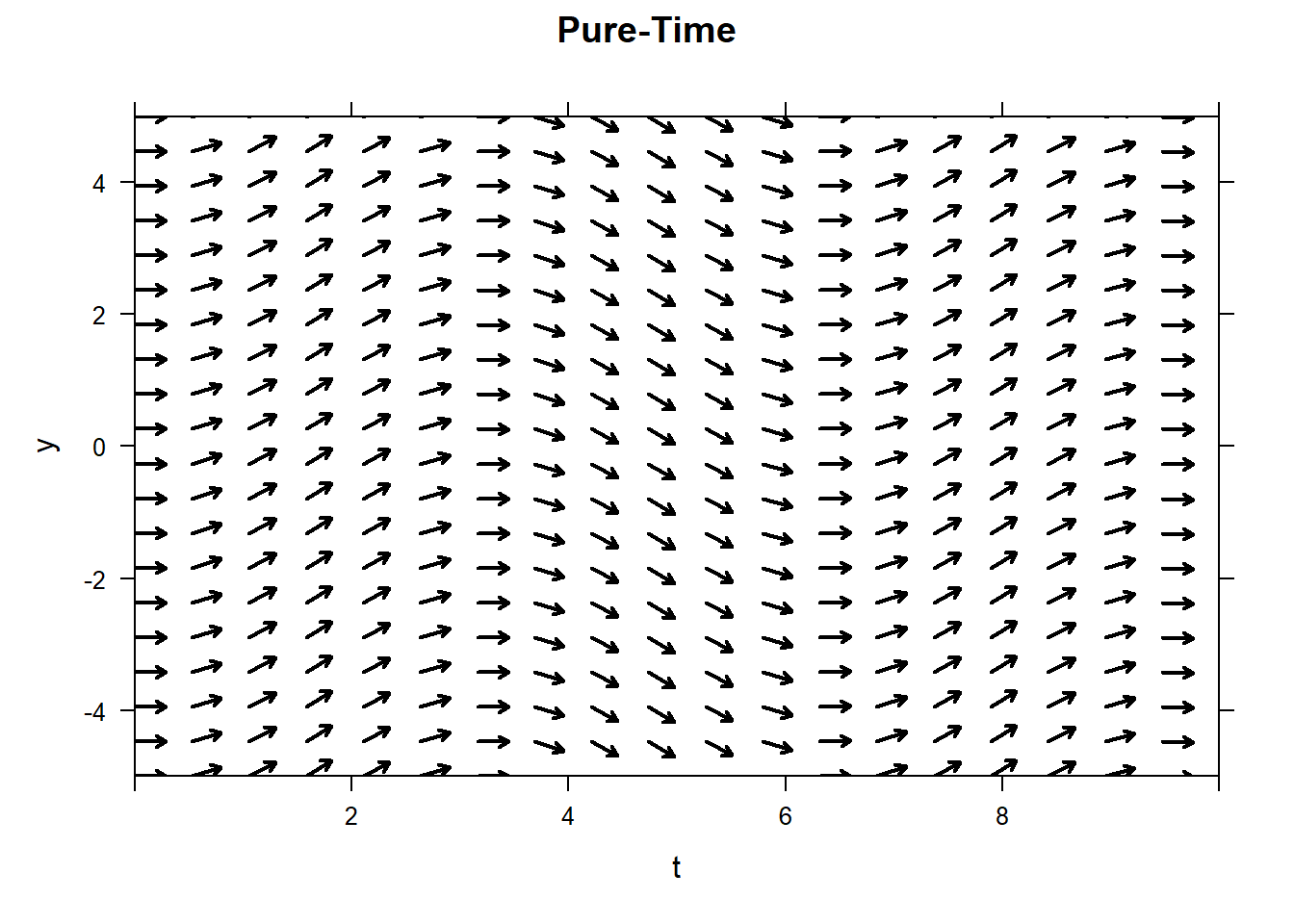

Practice identifying autonomous, pure-time, and neither ODEs from their corresponding direction field. Practice matching a direction field to an ODE. Exercises are in the chapter.